Precipitation Index
SPI & SPEI for Climate Extremes Monitoring
![]()
Monitor Climate Extremes with Confidence
A minimal, efficient Python implementation of Standardized Precipitation Index (SPI) and Standardized Precipitation Evapotranspiration Index (SPEI) for monitoring both drought and wet conditions using run theory.
Python 3.8+ BSD-3-Clause Active Development
Key Features
Climate Indices
- SPI — Standardized Precipitation Index
- SPEI — Precipitation Evapotranspiration Index
- Multiple time scales (1, 3, 6, 12, 24 months)
- CF-compliant NetCDF output
Bidirectional Analysis
- Monitor drought (dry conditions)
- Monitor floods (wet conditions)
- Unified framework for both extremes
- Consistent methodology
Multi-Distribution Fitting
- Gamma — Standard for SPI
- Pearson III — Recommended for SPEI
- Log-Logistic — Better tail behavior
- Automatic fitting method selection
Run Theory Framework
- Event identification & characterization
- Duration, magnitude, intensity, peak
- Time-series and gridded analysis
- Period statistics for spatial patterns
Operational Mode
- Save fitted distribution parameters
- Load and apply to new data without refitting
- Production monitoring workflows
- Validated identical to fresh calculations
Scalable Processing
- Memory-efficient spatial tiling
- Process global-scale data (CHIRPS, ERA5)
- Automatic memory estimation
- Streaming I/O for large datasets
Quick Example
import xarray as xr
from indices import spi
from runtheory import identify_events
from visualization import plot_index

# Load precipitation data
precip = xr.open_dataset('precipitation.nc')['precip']

# Calculate SPI-12
spi_12 = spi(precip, scale=12)

# Or use different distributions
spi_12_p3 = spi(precip, scale=12, distribution='pearson3')

# Identify drought events using run theory
events = identify_events(spi_12.isel(lat=0, lon=0), threshold=-1.2)

# Visualize
plot_index(spi_12.isel(lat=0, lon=0), threshold=-1.2)
from indices import spi, save_fitting_params, load_fitting_params
# Step 1: Calibrate on historical data and get parameters
spi_hist, params = spi(precip_historical, scale=12, return_params=True)
# Step 2: Save parameters for future use
save_fitting_params(params, 'spi12_gamma_params.nc',
scale=12, periodicity='monthly',
distribution='gamma',
coords={'lat': precip.lat.values,
'lon': precip.lon.values})
# Step 3: Later — load params and apply to new data (no refitting)
loaded = load_fitting_params('spi12_gamma_params.nc',
scale=12, periodicity='monthly',
distribution='gamma')
spi_new = spi(precip_new, scale=12, fitting_params=loaded)Why precip-index?
Calibrate distribution parameters on historical data, save them as NetCDF, and apply consistently to new observations — no refitting needed. This enables operational drought monitoring workflows where new satellite data is processed the moment it arrives, using the same statistical baseline every time. Validated to produce results identical to fresh calculations.
Benchmarked on a workstation with 128 GB RAM:
- CHIRPS v3 SPI-12 (0.05°, 17.3M cells, 539 months, ~69 GB) — ~2h 47m with Gamma distribution, 12 spatial chunks
- TerraClimate SPEI-12 (0.04°, 37.3M cells, 816 months, ~226 GB) — ~26h with Pearson III distribution, 32 spatial chunks
Regional subsets (country-level) complete in seconds to minutes. Memory-efficient spatial tiling means you don’t need a supercomputer. See Performance Benchmarks for detailed comparison.
WMO 11-category drought/wet classification. CF-compliant NetCDF output. Run theory from peer-reviewed hydrology literature. Multiple PET methods (Thornthwaite, Hargreaves) with automatic fallback. Three distribution families each using their optimal fitting method (Method of Moments, MLE, L-moments).
Global Output
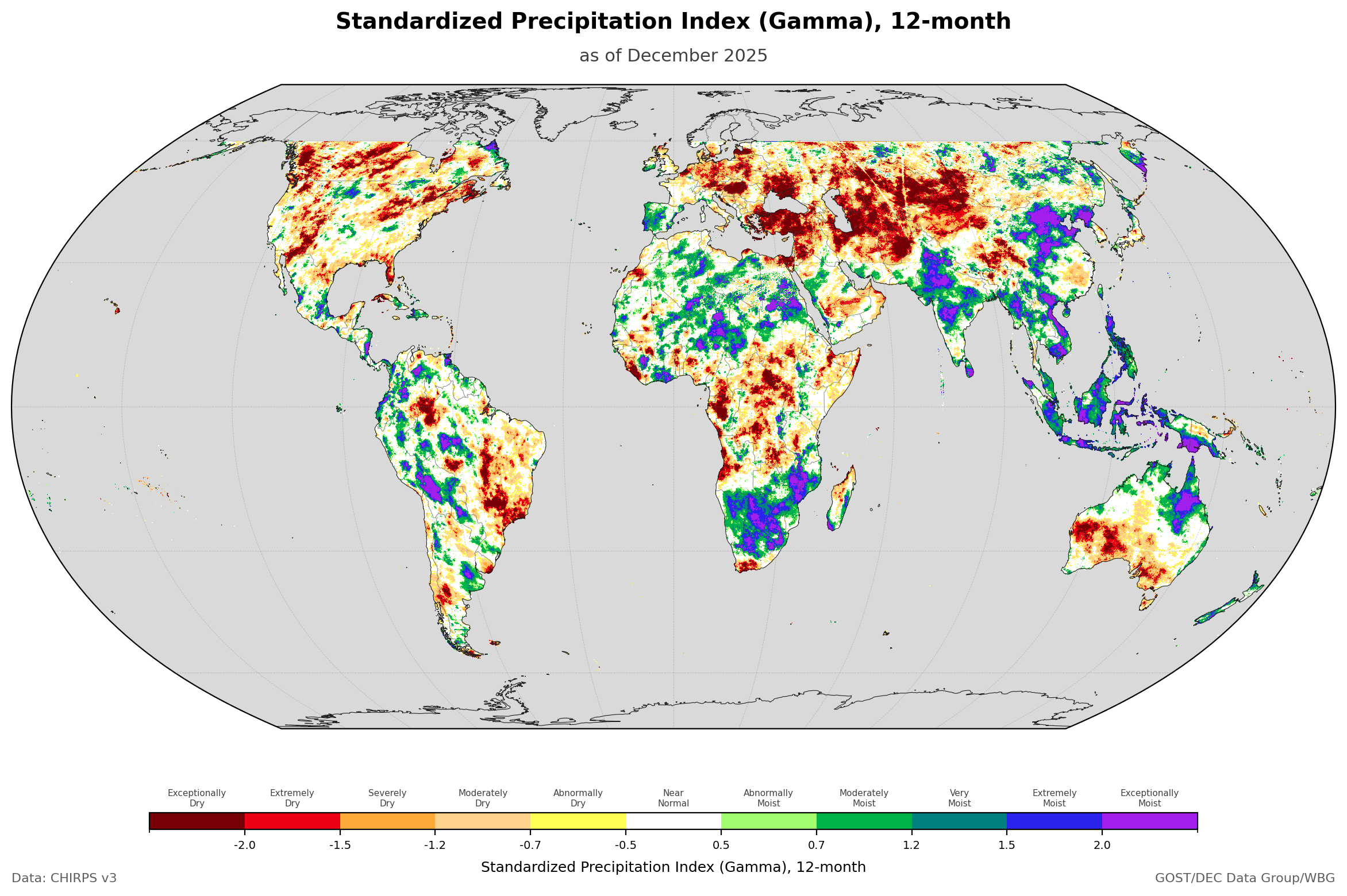
SPI-12 (Gamma) calculated from CHIRPS v3 at 0.05° resolution.
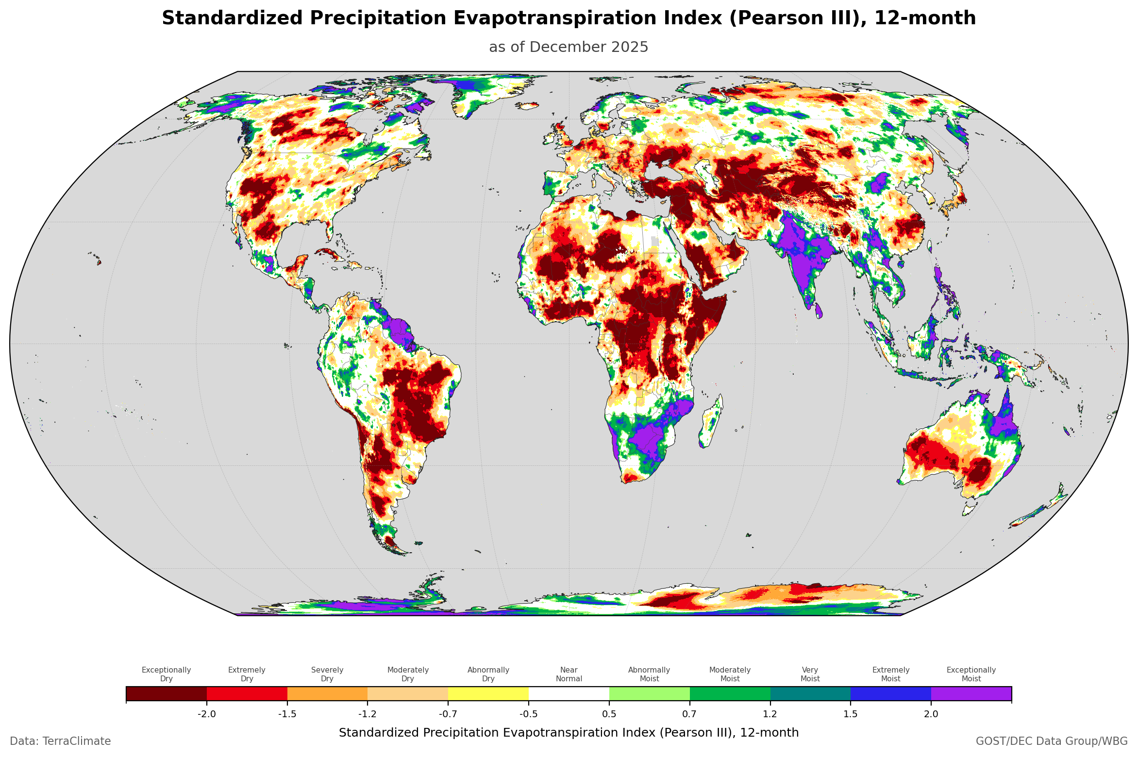
SPEI-12 (Pearson III) calculated from TerraClimate at 0.0417° ~ 4km resolution.
Validation Results
All distributions tested against TerraClimate Bali data (1958–2024). Cross-distribution correlation exceeds 0.98. The test suite generates 28 visualizations including advanced analytics and operational mode validation.
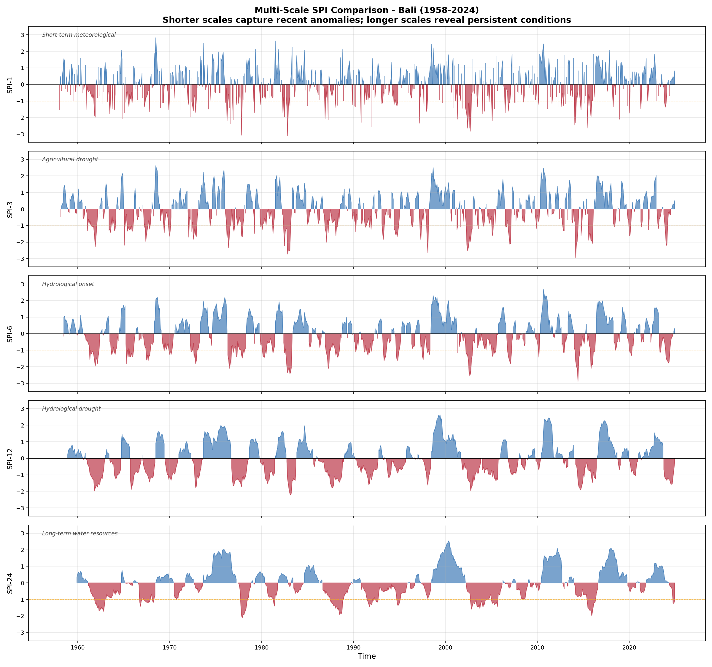
SPI at 1-, 3-, 6-, 12-, and 24-month scales. Each captures different drought types: meteorological, agricultural, hydrological, and socioeconomic.
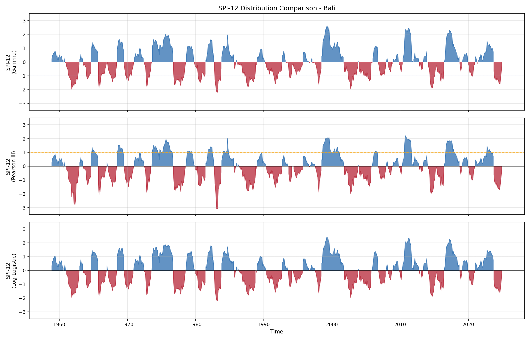
Three distributions produce consistent SPI-12 time series with correlation > 0.98 between all pairs.
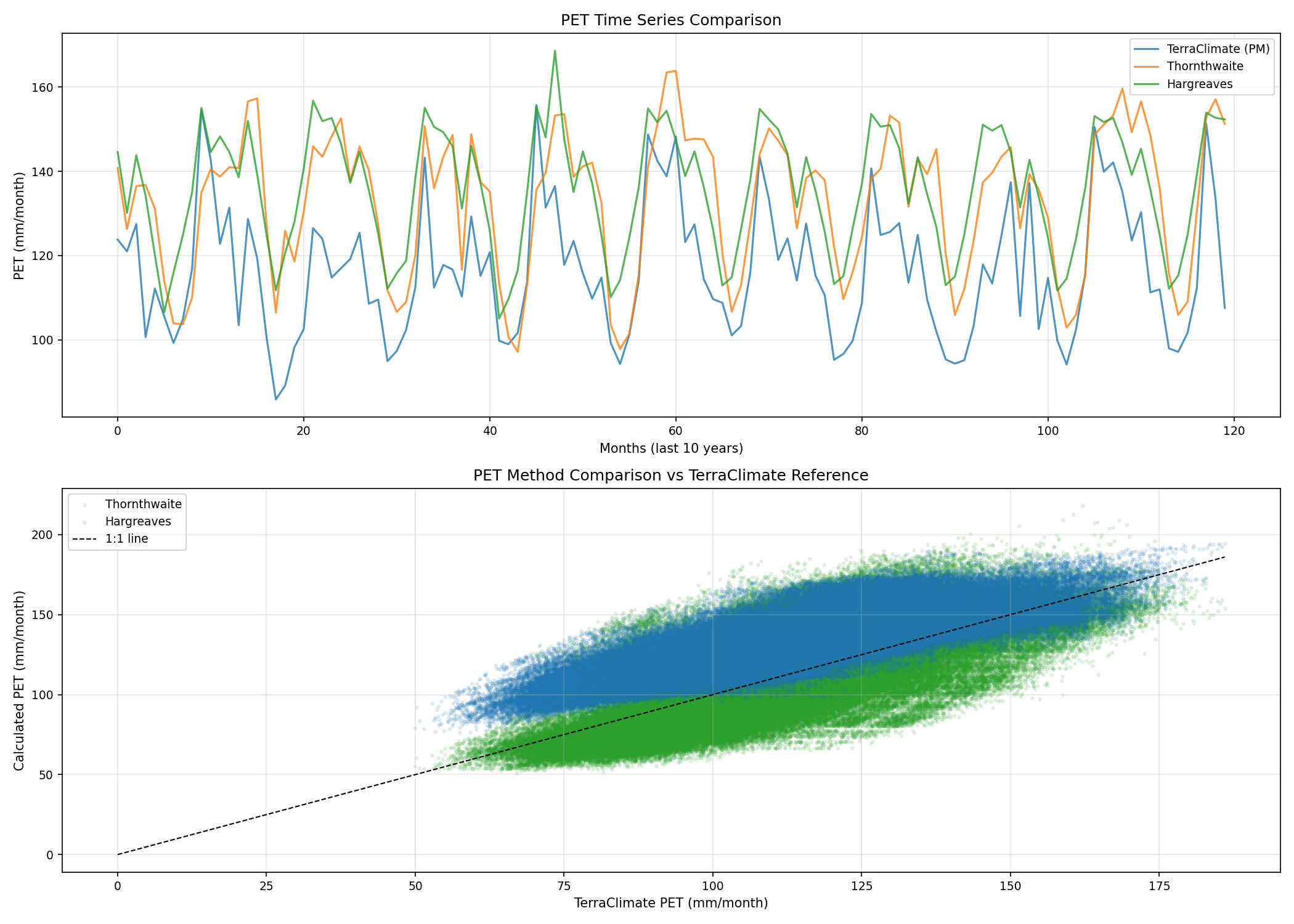
PET method comparison: Thornthwaite vs Hargreaves vs TerraClimate (Penman-Monteith). Hargreaves correlates better with the reference (r=0.80 vs r=0.75).
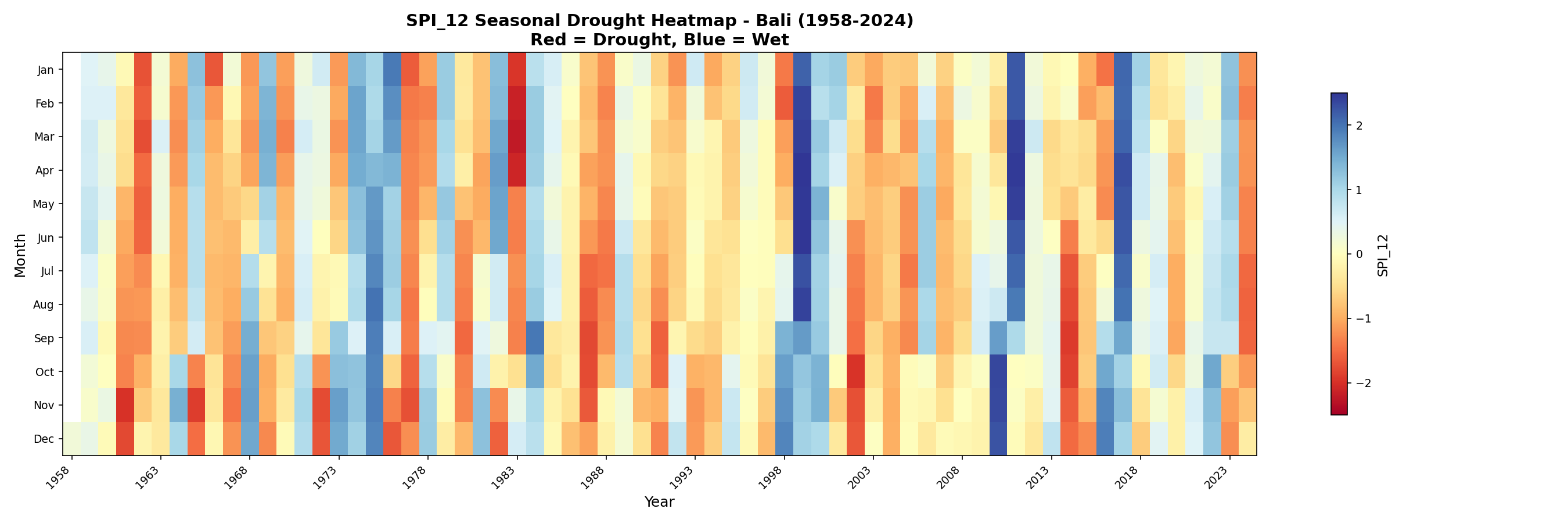
Seasonal drought heatmap showing month-by-year patterns. Major droughts (1997, 2015, 2019) appear as vertical red bands.
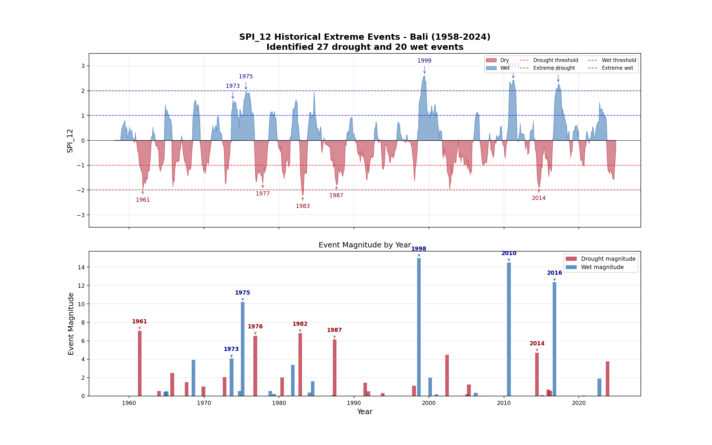
Run theory analysis identifies and ranks historical drought/wet events by magnitude.
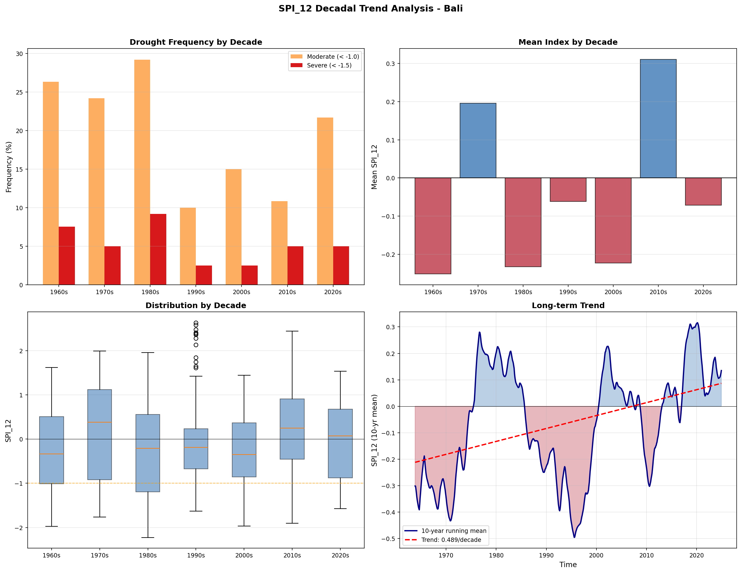
Long-term analysis showing drought frequency, mean index, and trends by decade.
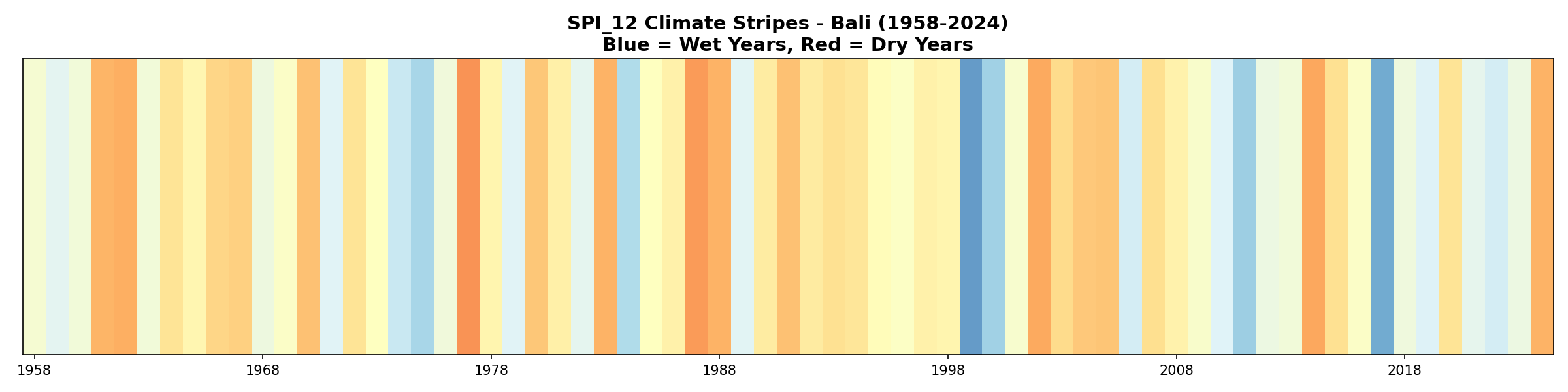
Climate stripes visualization showing annual drought conditions from 1959-2024. Red = drought years, blue = wet years.
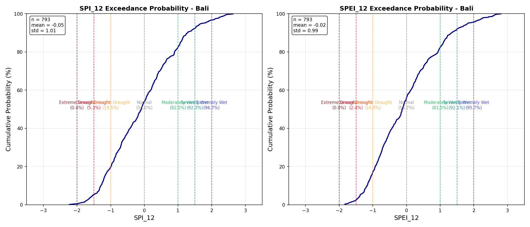
Risk assessment plot showing probability of exceeding drought thresholds with return period annotations.
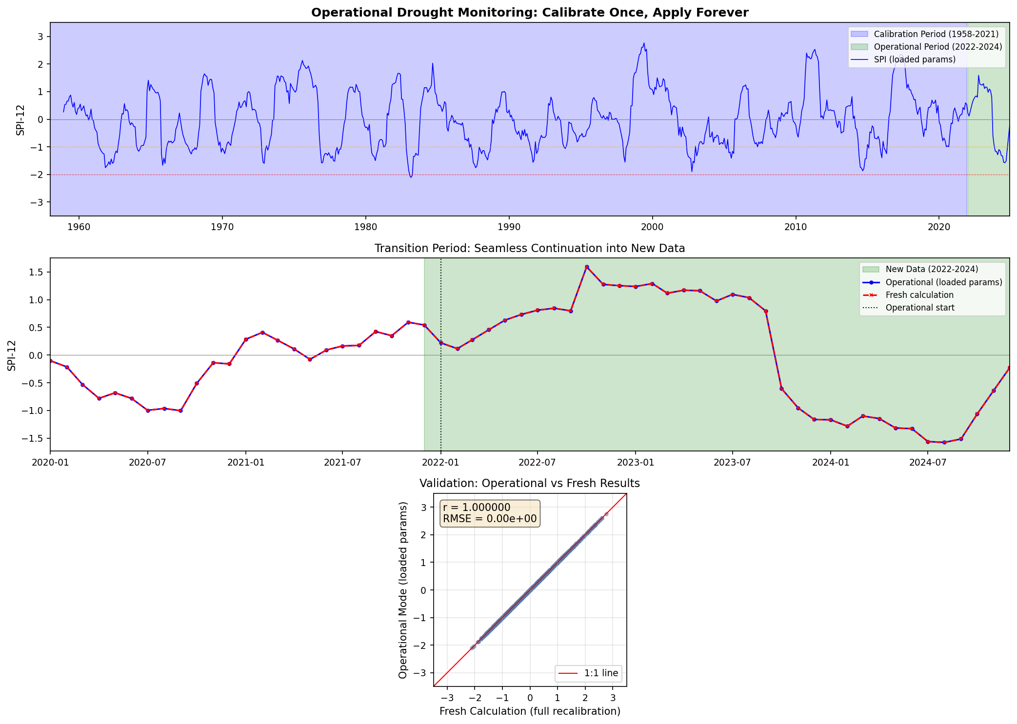
Parameter persistence for real-time monitoring: calibrate once on historical data, apply consistently to new observations. Results are identical to fresh calculations.
See Validation & Test Results for detailed analysis.
Getting Started
Installation
Install dependencies and clone the repository.
Quick Start
Calculate your first SPI/SPEI in minutes.
Tutorials
Learn through interactive examples with real data.
Documentation
- User Guide — SPI, SPEI, run theory, and visualization
- Technical Docs — Methodology, implementation, API reference
- Validation — Test results and comparison plots
- Changelog — Version history
Credits
Benny Istanto, GOST/DEC Data Group, The World Bank
Developed to support operational hydrometeorological monitoring — enabling the World Bank to regularly assess extreme dry and wet periods across regions.
Built upon the foundation of climate-indices by James Adams, with substantial modifications for multi-distribution support, bidirectional event analysis, and scalable processing.
Citation
@software{precip_index_2026,
  author = {Istanto, Benny},
  title = {Precipitation Index: SPI & SPEI for Climate Extremes Monitoring},
  year = {2026},
  url = {https://github.com/bennyistanto/precip-index},
  version = {2026.1}
}
Contributing & License
We welcome contributions! See our GitHub repository for bug reports, feature requests, and pull requests. Licensed under BSD-3-Clause.
This package is under active development. APIs may change. Please report issues on GitHub.