Full Pipeline

The same five notebooks drive both the Bali example and the full Indonesia run. The only difference is one line at the top of each notebook’s Step 1 cell:
CONFIG_FILE = 'config_bali.yml' # or 'config.yml' for full IndonesiaKeep all five notebooks (nb02 through nb06) on the same value when you switch.
The Bali subdomain
The shipped example runs on a small, fully reproducible slice of the grid: a 9 x 14 cell window at 0.1 deg over Bali, of which 80 cells are land and 46 are ocean-masked. Four BMKG stations fall inside it and serve as the independent validation set. This is what keeps the example light enough to run end-to-end in a Colab session while exercising every stage of the pipeline.
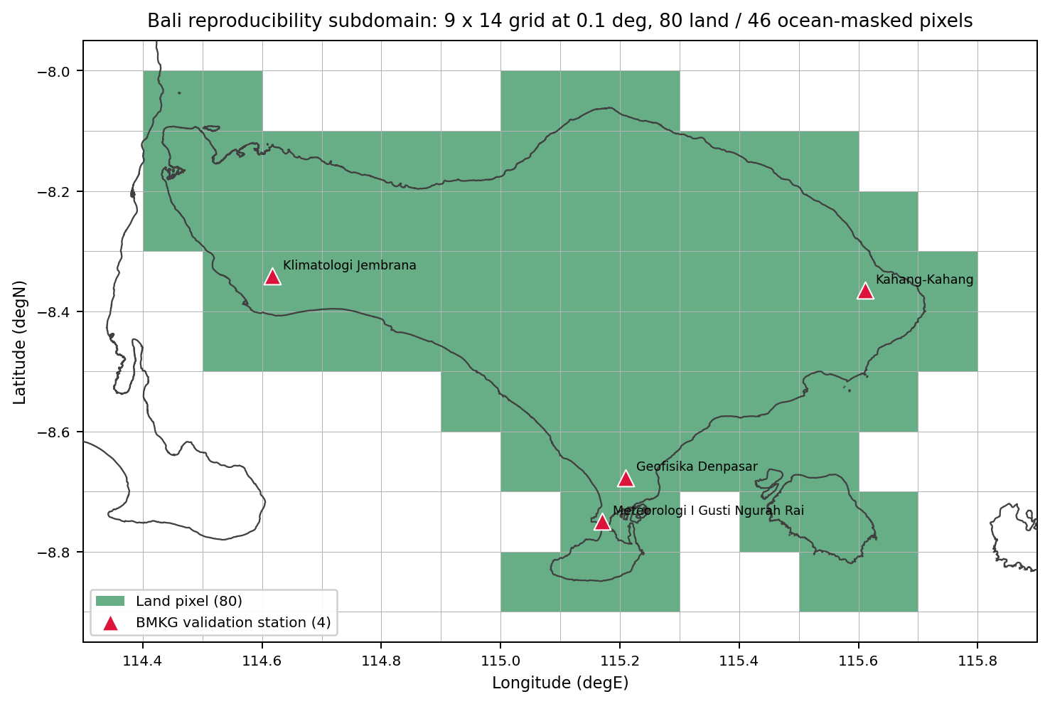
Notebooks involved
| Notebook | What it does |
|---|---|
00_define_aoi.ipynb, 01_data_acquisition.ipynb |
Region adaptation: define AOI + download IMERG / CPC. Skip for Bali (data ships with repo). Full walkthrough in Data Preparation. |
02_lseqmdl_bias_correction.ipynb |
LS → LSEQM → CNN train → DL blend, for all 36 dekads. |
03_measuring_performances.ipynb |
Computes metrics against CPC for each correction stage. |
04_qa_framework.ipynb |
Computes the Continuous Quality Index and writes per-period QA NetCDFs. |
05_station_validation.ipynb |
Independent validation against BMKG stations. |
06_visualisation_hub.ipynb |
Generates spatial figures + Taylor diagrams from the metrics / QA outputs. |
Step-by-step
- Step 1 of every notebook is the setup cell. It reads
CONFIG_FILEand callsinitialize_config(...). Edit this line to switch the AOI. - Step 2-5 (nb02) load IMERG / CPC / CPC-native / mask and pre-flight check the grids.
- Step 11 (nb02) is the batch loop. It calls
run_correction_pipeline(imerg_ds, cpc_ds, month, dekad, cpc_native_ds=...)fromsrc/bias_correction.pyfor each of the 36 dekads. - Step 7 (nb03) loops over
run_metrics_pipeline(month, dekad, mode)for each method -ls,lseqm,lseqmdl. - Step 6 (nb04) loops over
run_qa_pipeline(month, dekad, mode)to score each method. - Step 12 (nb05) runs the per-period station validation batch. If you skip Step 2 (data loading) and jump straight to the batch, the batch cell auto-loads
station_dfandobs_dfso it stays self-contained. - nb06 has individual visualisation cells plus a unified batch cell (Step 24) that runs all 4 visualisation batches (QA, QA regional, Taylor, station validation) in one go.
Each batch cell wraps every period in try/except so a single bad dekad does not block the rest.
Expected runtime
| Stage | Bali (Colab CPU) | Indonesia (local GPU, for reference) |
|---|---|---|
| nb02 batch (36 dekads, including CNN train) | 16.3 min | ~3-4 h |
| nb03 metrics | 45.4 min | ~30 min |
| nb04 QA | 6.9 min | ~30 min |
| nb05 station validation | 0.5 min | ~5 min |
| nb06 unified batch (all visualisations + Taylor) | 3.0 min | ~30-60 min |
| nb02 to nb06 total | 72.1 min |
The Bali column is measured, not estimated. nb03 dominates: metrics are computed for nine reference / method pairs per dekad. nb00 (AOI definition) and nb01 (download) are excluded, because both depend on the extent of the domain you request and on network throughput.
What you get out
After all notebooks finish, data/example_bali/output/ looks like this:
output/
  corrected_ls/         36 NetCDFs
  corrected_lseqm/      36 NetCDFs
  corrected_lseqmdl/    36 NetCDFs
  trained_models/       36 .keras models
  metrics_ls/           per-dekad metrics NetCDFs
  metrics_lseqm/        per-dekad metrics NetCDFs
  metrics_lseqmdl/      per-dekad metrics NetCDFs
  quality_ls/           per-dekad QA NetCDFs
  quality_lseqm/        per-dekad QA NetCDFs
  quality_lseqmdl/      per-dekad QA NetCDFs
  station_validation/   per-method CSVs (31 metrics + multi-threshold)
  station_density/      confidence_mask_station_density.nc4
  figures/
    qa/                 1296 PNGs (8 QA plot types x 36 periods x 2 modes
                                   + regional breakdowns)
    taylor/             152 PNGs (pooled + per-dekad Taylor diagrams)
    station_validation/ 288 PNGs (metric maps, threshold curves,
                                   regional box plots)
For a walkthrough of what the figures look like and how to read them, see the QA Framework and Station Validation tutorials.
Memory on Colab
The batch cells are memory-aware:
_load_corrected(Taylor pipeline) opens NetCDFs with awithblock so file handles are released immediately.- Every batch loop ends each iteration with
plt.close('all')andgc.collect()so the previous period’s arrays and matplotlib state are freed before the next period loads. - Admin boundary shapefiles are loaded once per session, clipped to the AOI, and cached as numpy line segments (about 3-4 MB for Bali).
If you still hit OOM on a larger AOI, the most likely cause is the CNN training step in nb02 (TensorFlow can pin memory across calls). Adding tf.keras.backend.clear_session() between dekads usually resolves it.