Station Validation

CPC-UNI is the training reference. The BMKG stations are not in the CPC pipeline (different national agency, different processing), so they provide an independent check on the bias correction.
For the Bali example bundle there are 4 BMKG stations:
| WMO ID | Name | Lat | Lon | Elev (m) |
|---|---|---|---|---|
| 97230 | I Gusti Ngurah Rai (airport) | -8.75 | 115.17 | 4 |
| 97232 | Geofisika Denpasar | -8.68 | 115.21 | 15 |
| 97234 | Kahang-Kahang | -8.37 | 115.61 | 155 |
| 97236 | Klimatologi Jembrana | -8.34 | 114.62 | 25 |
What nb05 does
The batch cell (Step 12) iterates the 36 dekads. For each one:
- Loads the per-dekad corrected NetCDFs (LS, LSEQM, LSEQM+DL).
- Extracts the value at each station’s nearest pixel.
- Pairs against the BMKG daily observations, filtering missing values (sentinel
8888.0). - Computes the 31 WMO-style metrics per station, plus the multi-threshold POD / FAR / CSI table.
- Saves CSVs under
output/station_validation/.
If you skip Step 2 (which loads station_df and obs_df interactively) and jump straight to the batch cell, it now auto-loads those variables - the batch is self-contained.
Single-station diagnostics
Two on-demand views are useful before looking at the regional / Taylor summaries below. The figures here are pinned to the four BMKG stations available in the Bali bundle:
| WMO | Station | Setting |
|---|---|---|
| 97230 | I Gusti Ngurah Rai | Coastal airport, southern Bali |
| 97232 | Geofisika Denpasar | Urban, central south |
| 97234 | Kahang-Kahang | Inland (155 m elev), eastern Bali |
| 97236 | Klimatologi Jembrana | Western Bali, near coast |
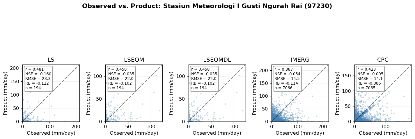
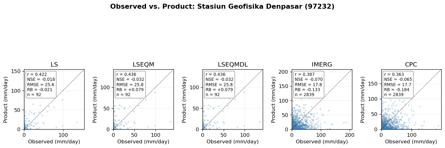
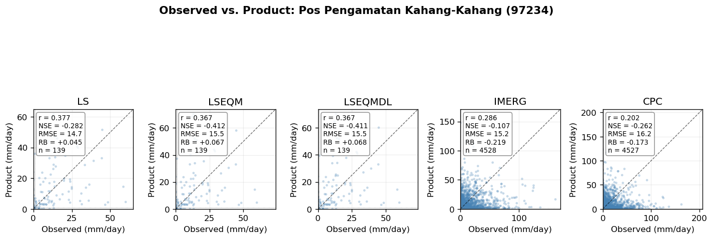
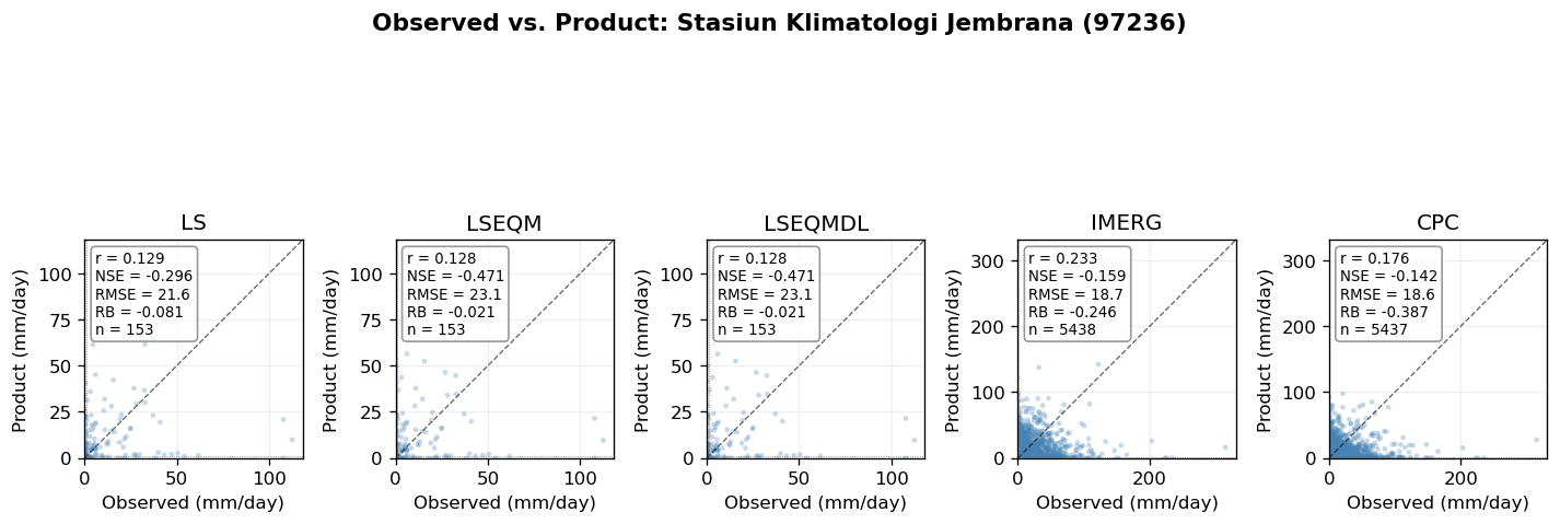
Comparing the four lets you see how the framework behaves under different exposures (coastal vs inland, dense vs sparse local rain).
Per-station scatter against BMKG
Step 8 plots BMKG observed vs each corrected product on the same axes, with 1:1 reference and per-product r / RMSE / NSE annotations. It surfaces the dry-bias floor in IMERG-L and the progressive tightening of the cloud as LS → LSEQM → LSEQM+DL are applied.
Daily time series
Step 9 plots the daily series as dots (not lines, so missing days do not get interpolated visually). Black = BMKG observed across the full 2001-2021 gauge record; the colored cluster is the January dekad 1 corrected series, set against IMERG and CPC as full-period baselines. WMO intensity thresholds (5, 10, 20, 50, 100 mm/day) are overlaid as horizontal references.
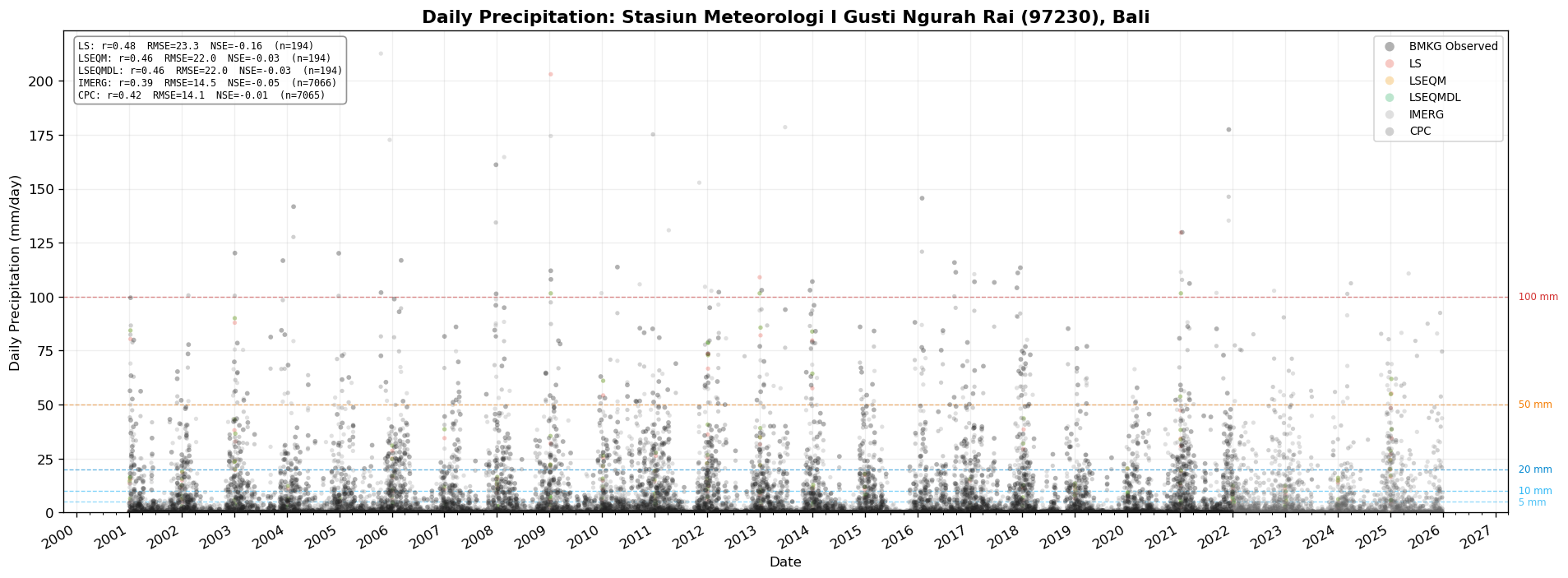
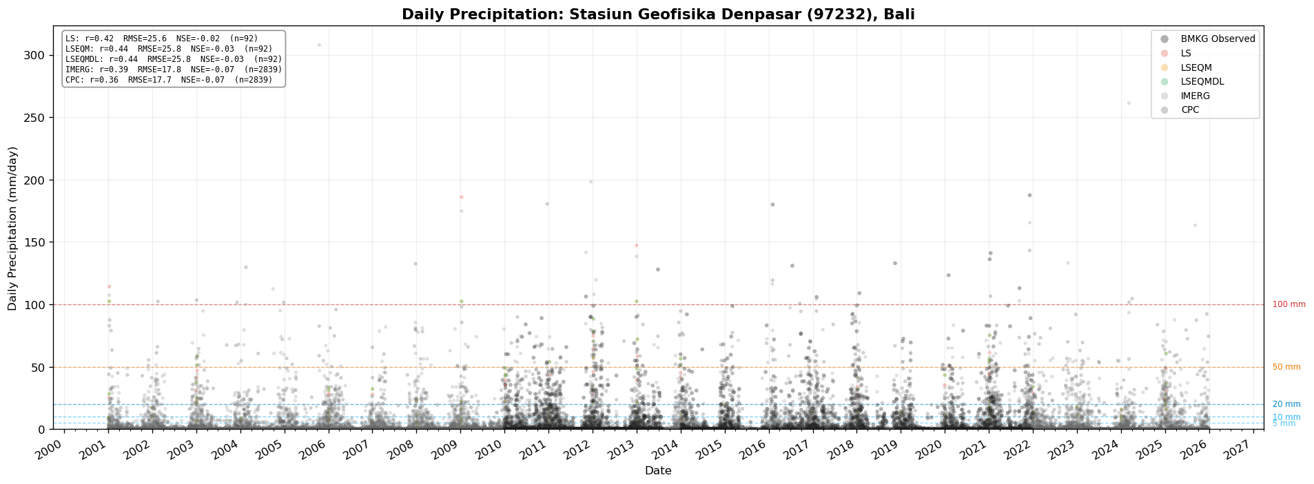
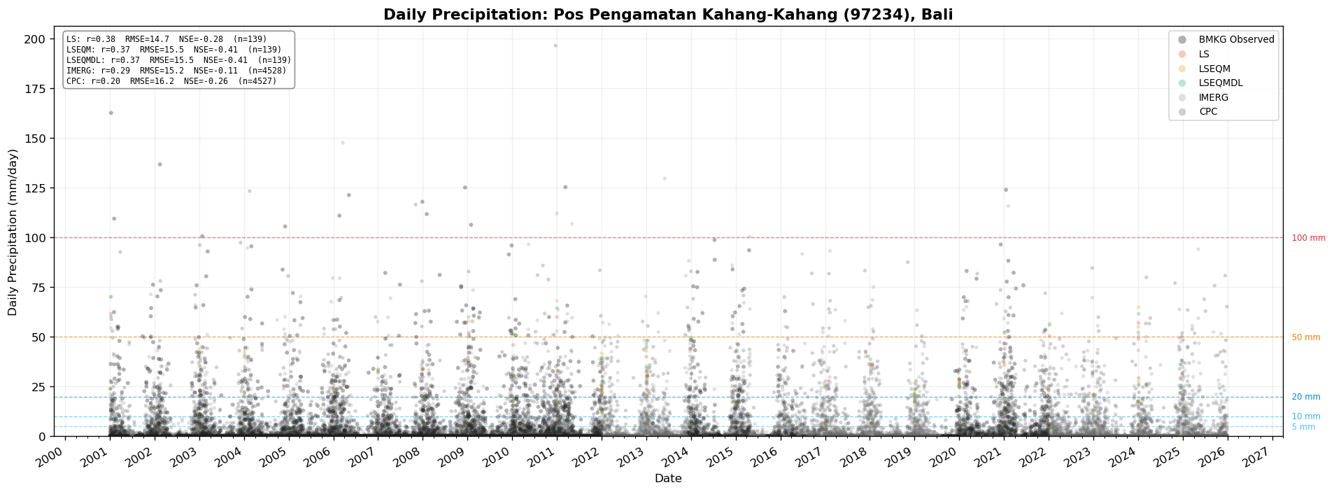
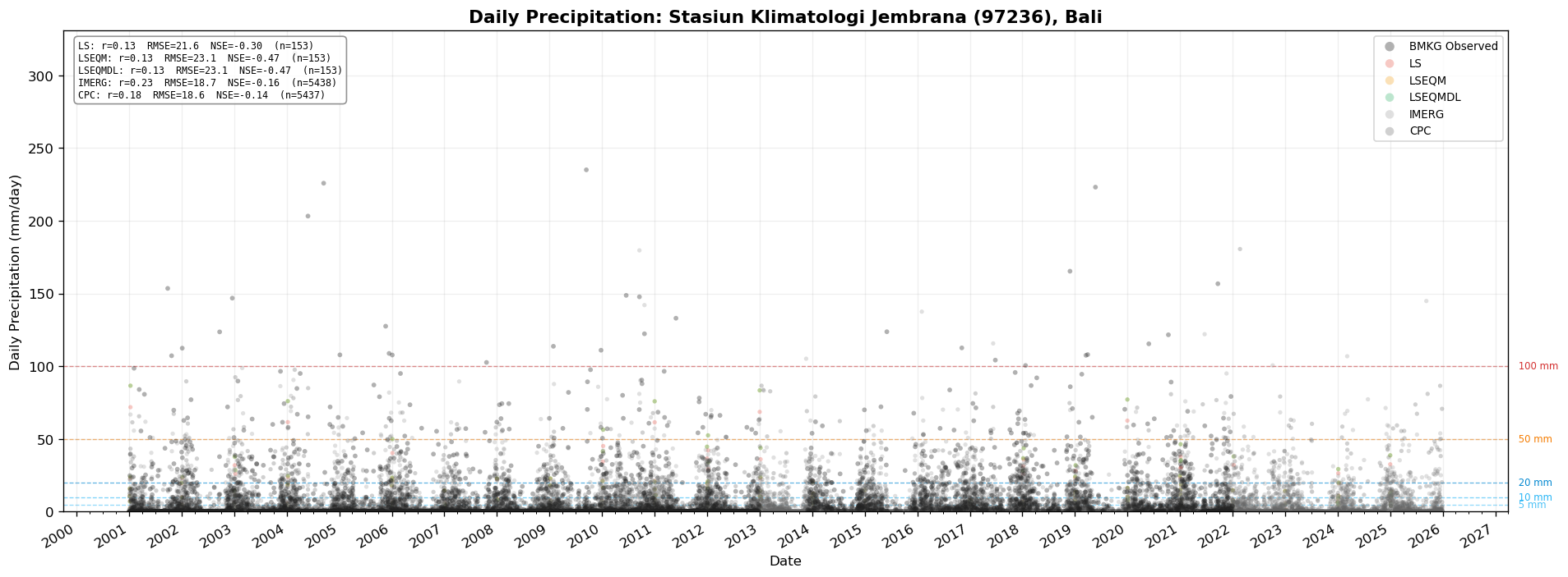
Source: nb05 Step 9 - Per-Station Daily Precipitation Time Series
The notebook supports any station in the loaded obs_df. The figures above are pinned to Bali; for other AOIs, change STATION_WMO_ID in nb05 Steps 8 / 9 and re-run.
What nb06 then plots
The nb06 station-validation batch reads the CSVs from nb05 and writes the figures discussed below.
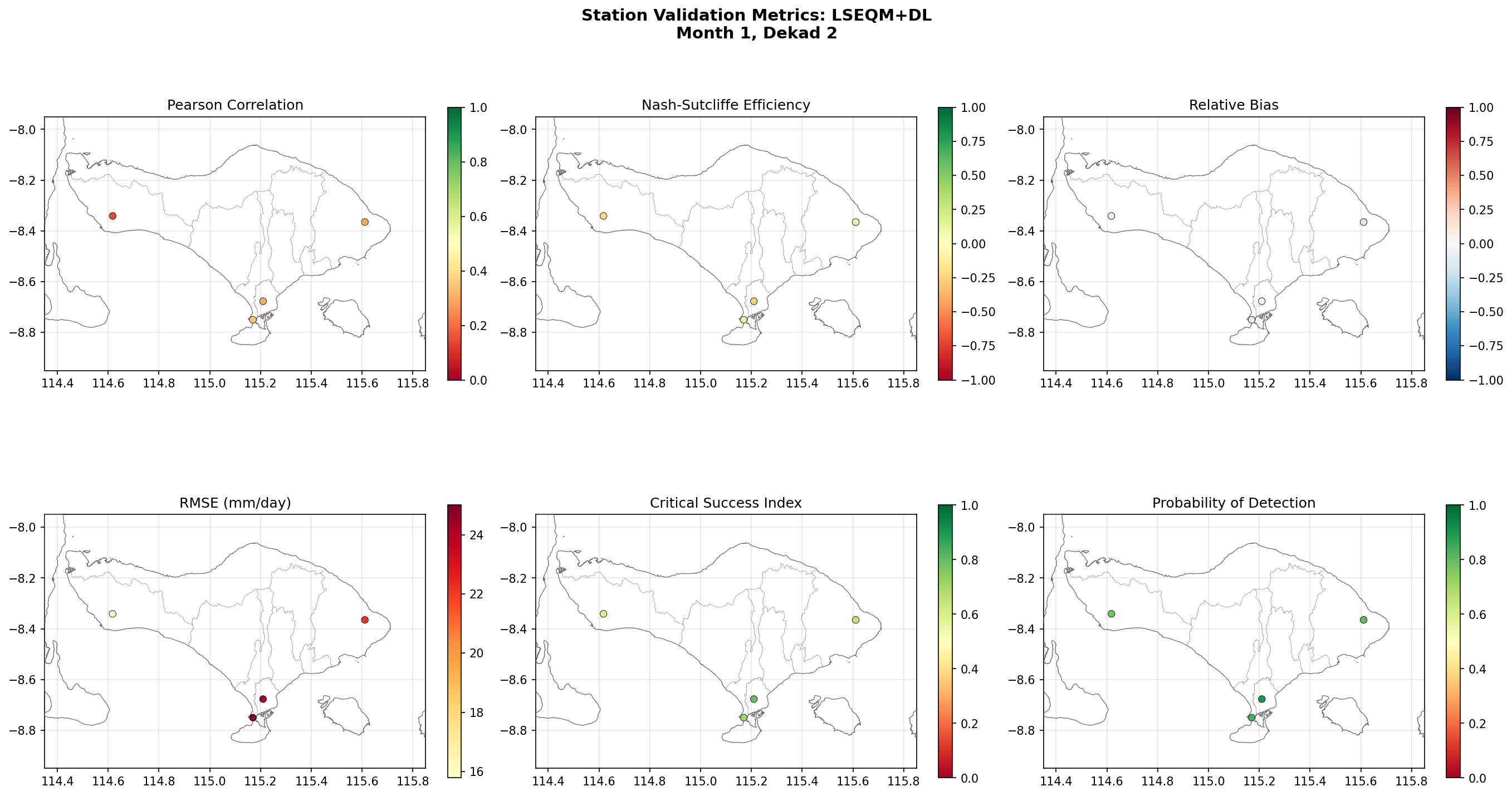
Per-station metric scatter maps
One 2 × 3 panel of key metrics across all stations, per method. Bali, January dekad 11-20, LSEQM+DL:
Source: nb06 Step 21 - Station Metric Scatter Maps
The dot colour at each station encodes the metric value; the dot position is the station location. Bigger dots, or warmer / cooler colours away from neutral, flag stations where the method does poorly.
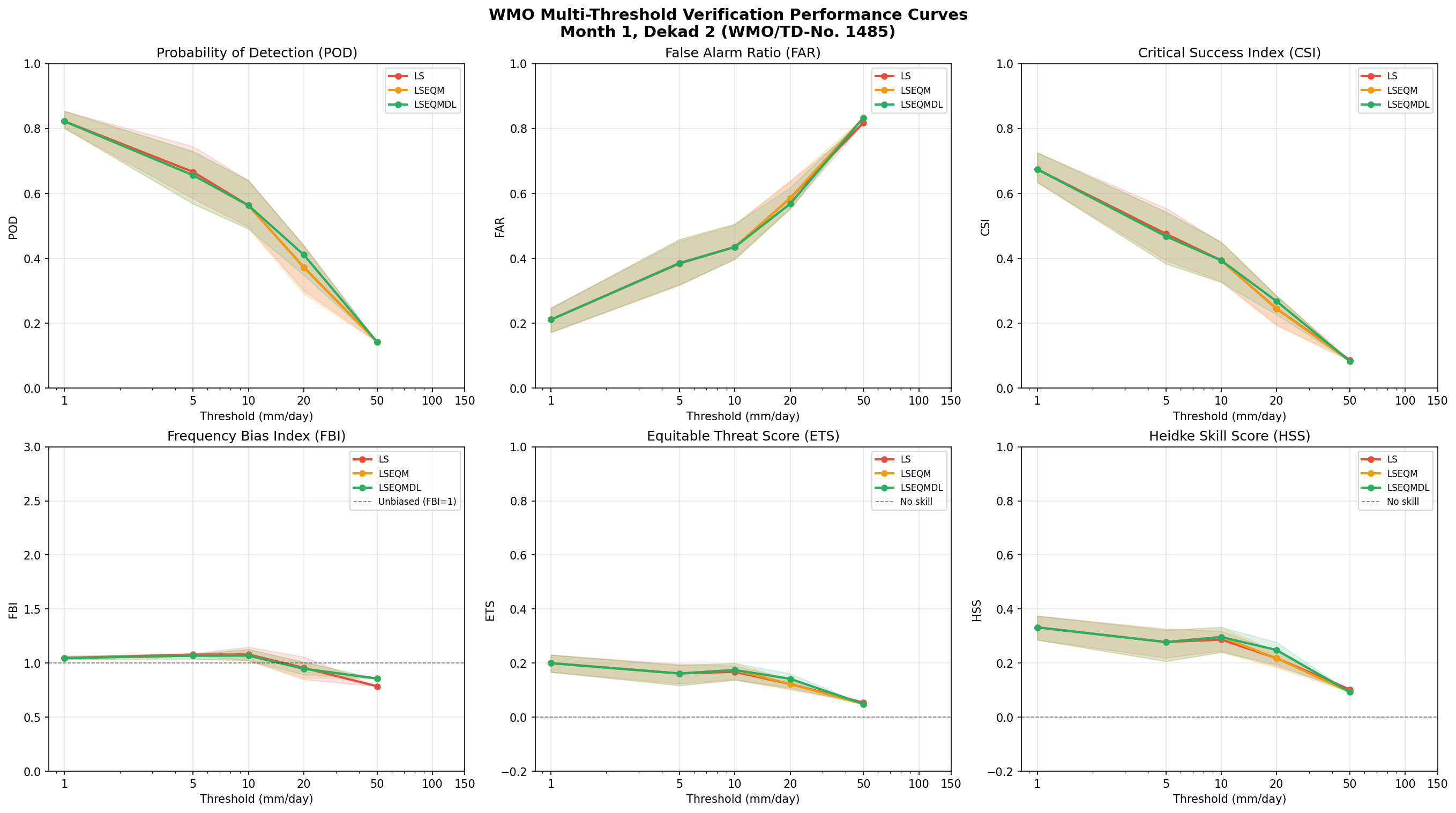
Multi-threshold WMO curves
POD / FAR / CSI computed at WMO thresholds (1, 5, 10, 20, 50, 100, 150 mm) for each method:
Source: nb06 Step 22 - Multi-Threshold Performance Curves
This is where the categorical impact of each correction stage is clearest: light-rain thresholds show LS already does most of the work; heavy-rain thresholds (20-50 mm) is where LSEQM+DL earns its keep.
The Bali curve stops at 50 mm because the 4-station Bali sample doesn’t accumulate enough observed events at 100 / 150 mm to pass the WMO/TD-1485 10-event minimum (per-station CSVs report NaN for those thresholds, and the plot drops empty levels). The framework still computes them; they populate when run against the full 172-station validated Indonesia network. See FAQ - Why does the Bali multi-threshold curve only show up to 50 mm?
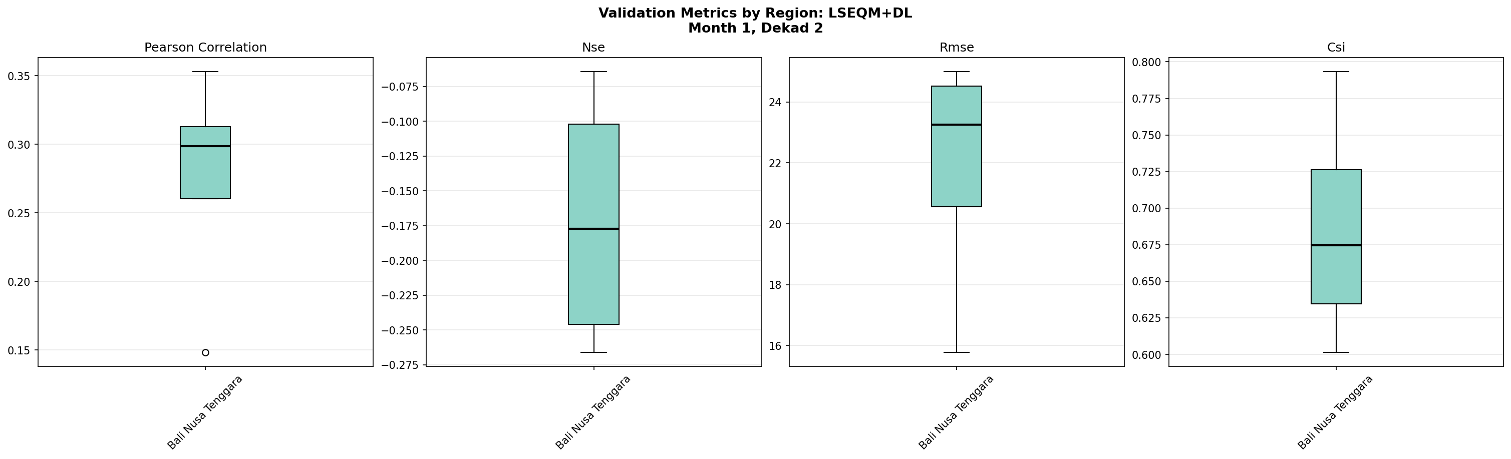
Regional box plots
Regional aggregation collapses the per-station metrics by region_mapping (Sumatra, Jawa, Kalimantan, Sulawesi, Bali Nusa Tenggara, Maluku, Papua). For Bali the only region is “Bali Nusa Tenggara”:
Source: nb06 Step 23 - Regional Box Plots
For the full Indonesia run, this view becomes much more interesting - it surfaces where the framework performs well and where it does not.
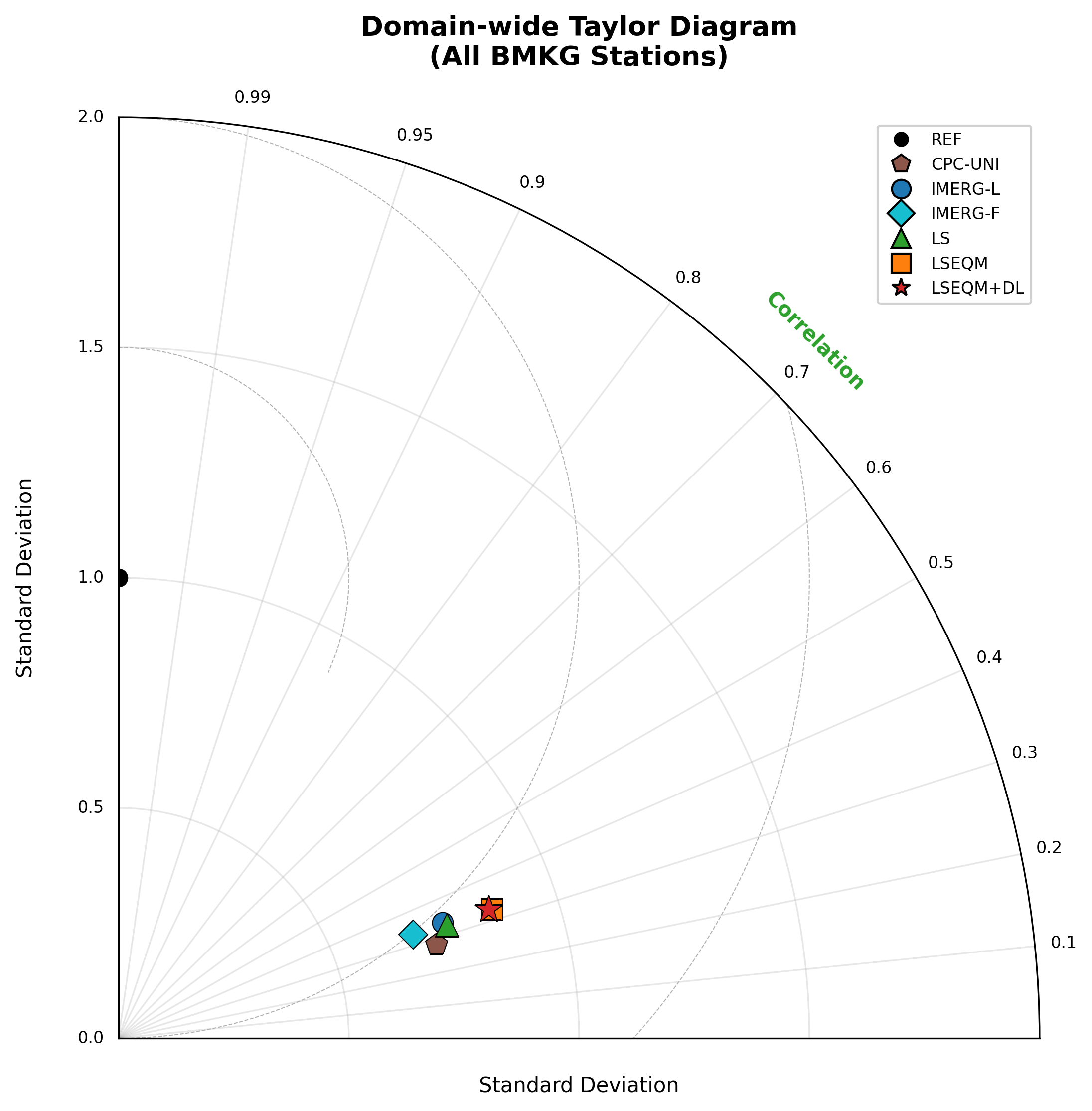
Taylor diagrams (from nb06)
nb06’s Taylor pipeline (compute_all_taylor_stats + generate_*_taylor) pairs each product against each BMKG station’s daily record across the entire 2001-2021 gauge period, then plots the median.
Domain-wide Taylor (pooled across all stations):
Source: nb06 Step 13 - Domain-Wide Taylor Diagram
By-island (only Bali Nusa Tenggara for the Bali example; this becomes a real multi-panel figure on Indonesia):
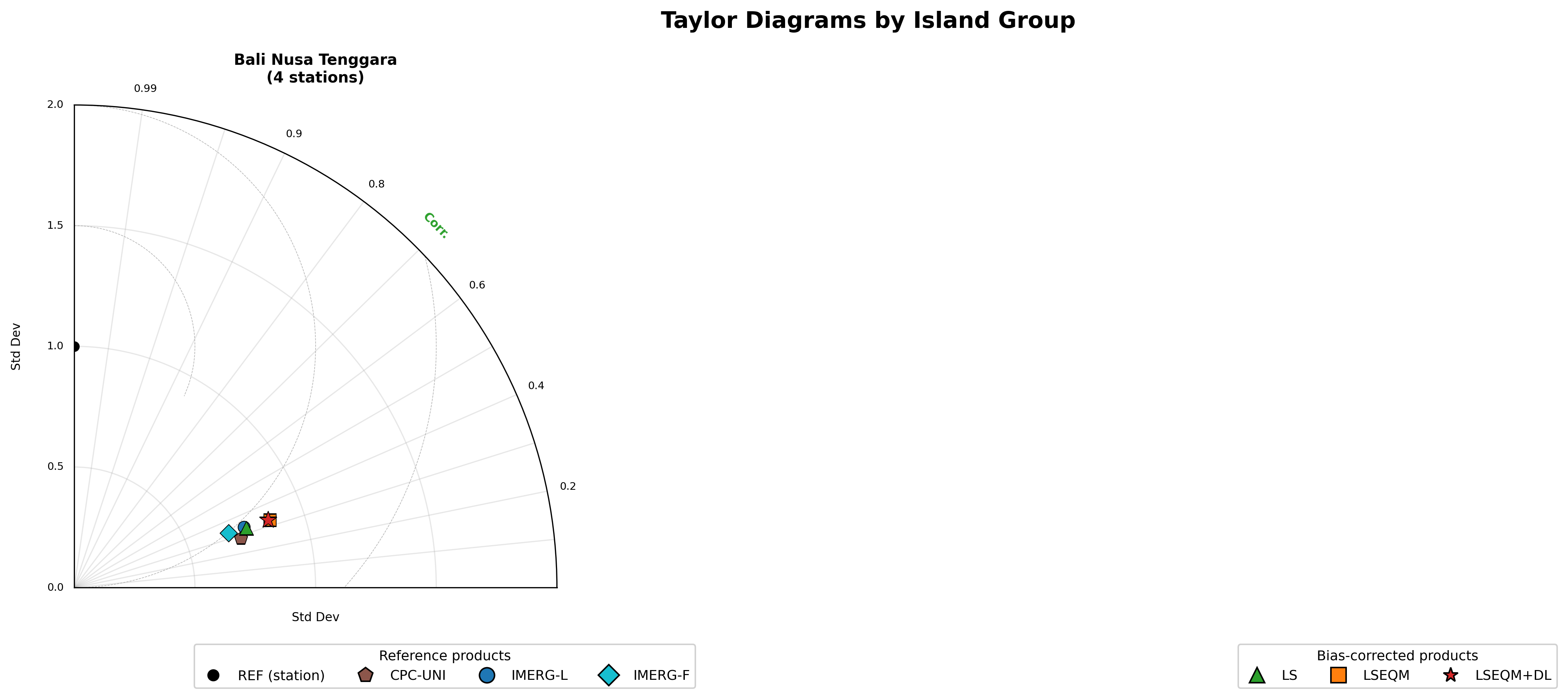
Source: nb06 Step 14 - Taylor Diagrams by Island Group
Per-station Taylor (one marker per station, with the cluster median as a larger marker):
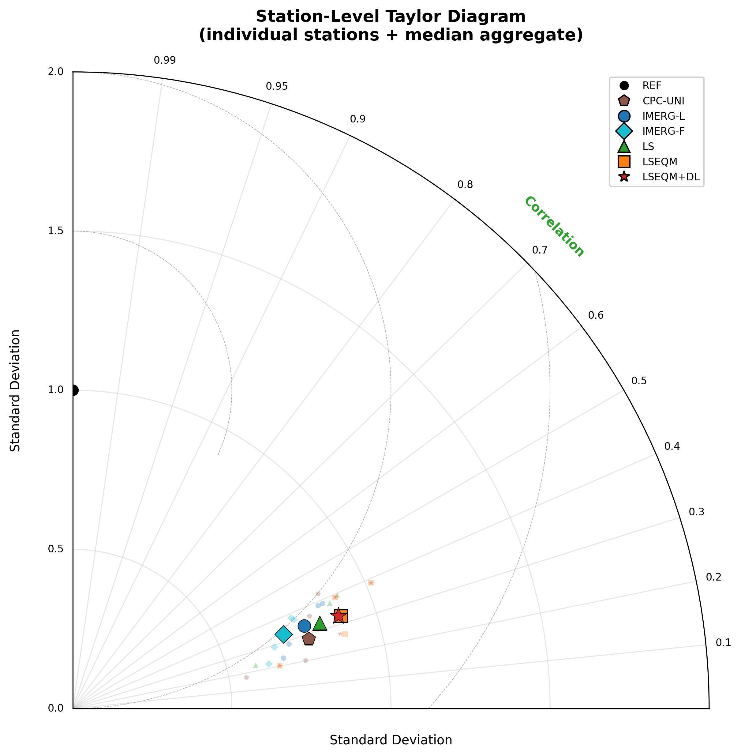
Source: nb06 Step 16 - Station-Level Taylor Diagram
The Taylor design follows the paper figure: bottom “Standard Deviation” axis label, “Correlation” label at 45 degrees close to the outer arc, denser correlation ticks at 0.95+ with 2-decimal formatting, and a split legend (reference products vs bias-corrected products) anchored at the bottom of the figure.
Reading the diagrams
Each point encodes three things:
- Angle from the y-axis = Pearson correlation (closer to the vertical = higher correlation, ranging 0 to 1).
- Radius = standard deviation ratio (1.0 = matches the observed variability; <1 underestimates; >1 overestimates).
- Distance from the reference point at (0, 1.0) = centred RMSE (lower = better).
Movement toward the reference point as you go from IMERG-L → LS → LSEQM → LSEQM+DL is the desired pattern.
Headline numbers
Quantitative headline numbers from the full-Indonesia run across the 172 validated BMKG stations will be filled in here when the companion paper is finalised. The Bali bundle’s 4-station numbers are useful for sanity-checking the toolchain but are not statistically robust on their own.