QA Framework

The Continuous Quality Index (CQI) is a single 0-1 score per pixel that summarises how well a corrected field reproduces the reference. It is the weighted sum of three component scores:
\[ \text{CQI} = w_b \cdot S_{\text{basic}} + w_d \cdot S_{\text{dist}} + w_t \cdot S_{\text{temporal}} \]
with default weights \(w_b = 0.4\), \(w_d = 0.3\), \(w_t = 0.3\).
The full roll-up is a two-level tree: 31 raw metrics collapse into three normalised sub-scores, which collapse into the single CQI. The weights below are read directly from config.yml (the three component weights) and src/qa_framework.py (the within-component weights), so the figure and the code cannot drift:
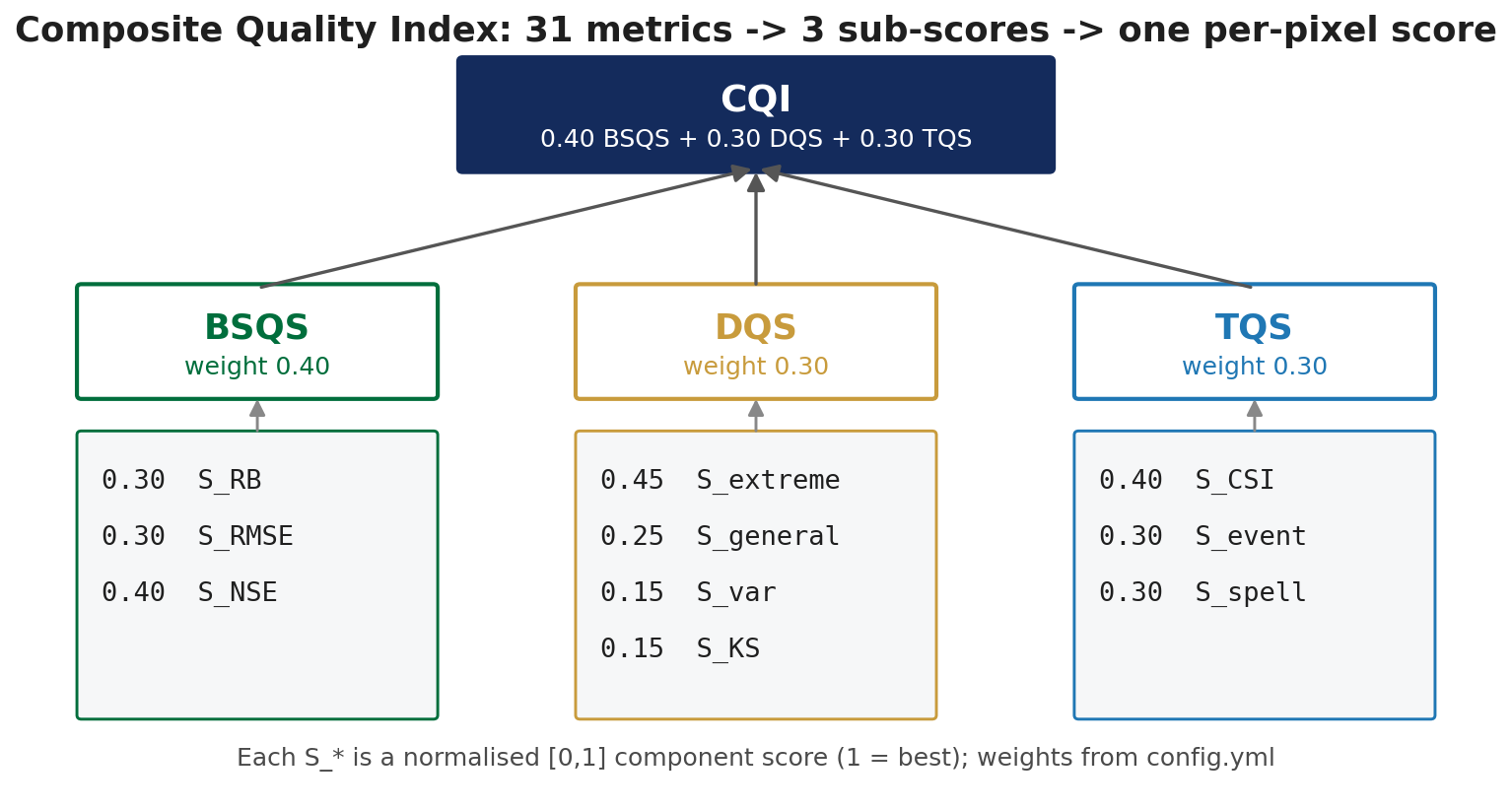
config.yml; within-component weights from src/qa_framework.py.
The components
| Component | What it measures | Scored metrics (within-component weight) |
|---|---|---|
| Basic | Mean bias and amplitude error | relative bias (0.30), RMSE (0.30), NSE (0.40) |
| Distribution | Whether the full distribution shape is corrected, not just the mean | extreme percentiles p90/p95/p99 (0.45), general percentiles p25/p50/p75 (0.25), std-dev ratio (0.15), KS test (0.15) |
| Temporal | Whether event timing and dry spells are preserved | CSI (0.40), event timing = POD and 1-FAR (0.30), dry-spell length (0.30) |
Each component is normalised to [0, 1] before weighting; the within-component weights above are the ones drawn in the tree figure and set in src/qa_framework.py.
Pearson correlation is deliberately not folded into the CQI. It is reported separately, alongside RMSE and NSE, as a timing diagnostic. This is the design choice that keeps the correlation ceiling visible: had daily r been averaged into a composite score, the flat-correlation result would have been masked.
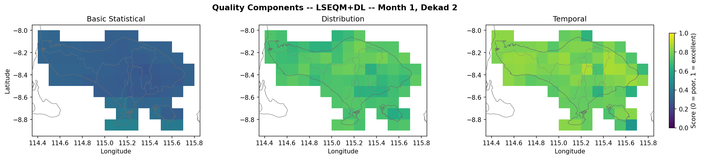
Component scores side-by-side
Bali, January dekad 11-20, LSEQM+DL. Higher = better:
Categorical bands
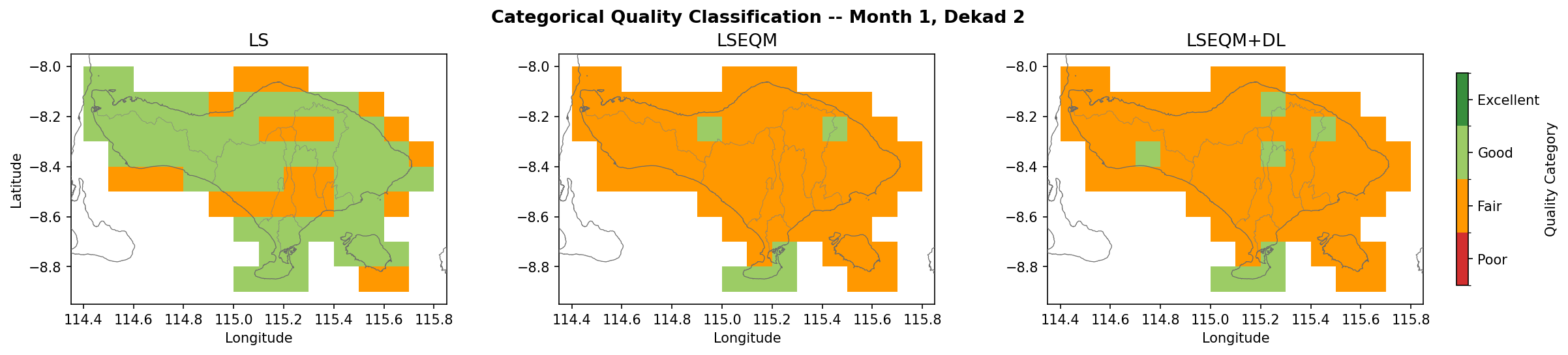
| CQI range | Class | Reading |
|---|---|---|
| >= 0.80 | Excellent | Correction reproduces the reference closely |
| >= 0.60 | Good | Main features captured, minor discrepancies |
| >= 0.40 | Fair | Improves on raw satellite, significant biases remain |
| < 0.40 | Poor | Correction fails to improve or degrades the satellite estimate |
Spatial CQI maps
For each dekad and each method, 04_qa_framework.ipynb writes a quality_{method} NetCDF with the CQI and its three component fields. The visualisation hub (nb06) renders them as three-panel comparisons.
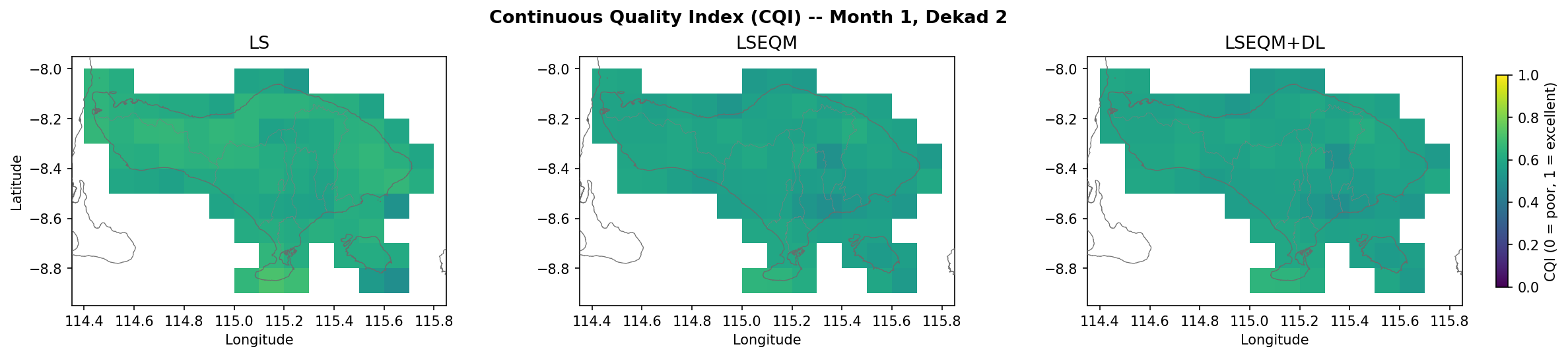
Source: nb06 Step 4 - CQI Spatial Maps
The categorical version uses the bands above:
What the DL stage actually moves
The improvement map (LSEQM+DL minus LS) shows where the deep-learning stage shifts the score:
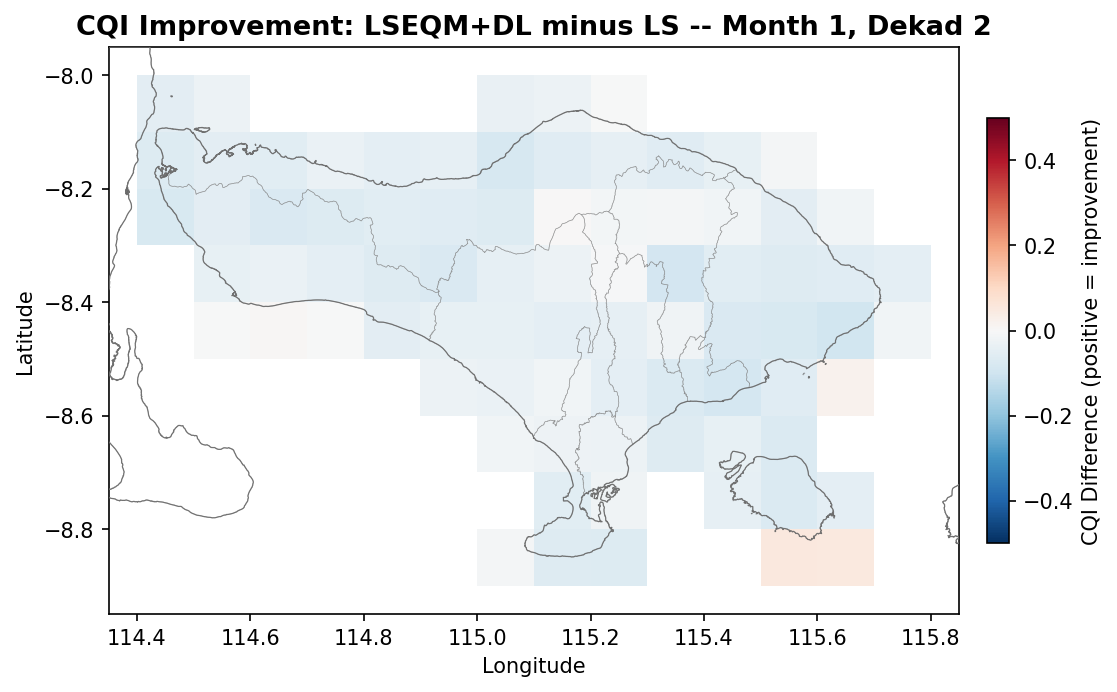
Source: nb06 Step 6 - Method Improvement Map
In gauge-dense areas, the DL stage usually adds a small but consistent improvement. In gauge-sparse areas, the station-density confidence mask returns the result to LSEQM, so the improvement is zero by construction. The confidence map shows where each pixel sits on that scale:
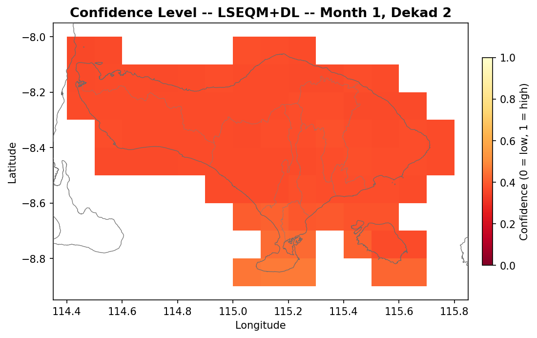
Source: nb06 Step 8 - Confidence Map
Distribution and box plots
CQI distribution shows the histogram and CDF of pixel scores per method:
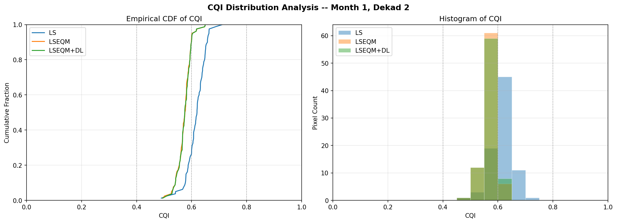
Source: nb06 Step 9 - CQI Distribution Analysis
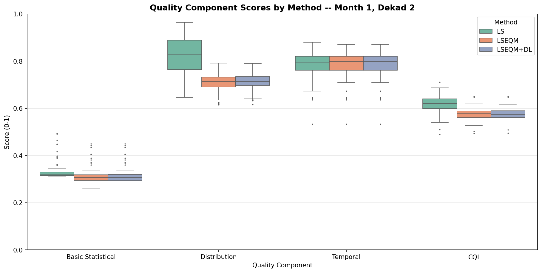
Per-component box plots compare LS / LSEQM / LSEQM+DL on each component separately:
Interpreting changes between methods
The expected pattern, in tropical settings:
- LS improves the mean - basic score jumps from raw IMERG.
- LSEQM lifts the distribution component substantially - this is where the Gamma + GPD fit pays for itself.
- LSEQM+DL adds small gains in the basic component over densely gauged areas, and is neutral elsewhere by design (the confidence mask returns those cells to LSEQM).
If LSEQM+DL is worse than LSEQM in data-sparse cells, the confidence mask is probably misconfigured. Check saturation_count and inspect confidence_mask_station_density.nc4 under output/station_density/.
For Bali specifically, all four BMKG stations sit in the southern half of the island, so the confidence mask is highest in southern Bali and near-zero over the northern coast.