Blending
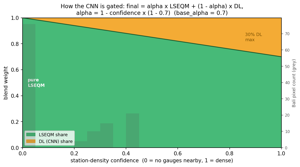
The final LSEQM+DL field is a per-pixel weighted average of the LSEQM field and the CNN output, with the weighting controlled by the station-density confidence mask.
The formula
For each pixel \((i, j)\):
\[ P^{LSEQMDL}_{i,j} = \alpha_{i,j} \cdot P^{LSEQM}_{i,j} + (1 - \alpha_{i,j}) \cdot P^{CNN}_{i,j} \]
where the effective alpha is:
\[ \alpha_{i,j} = 1 - c_{i,j} \cdot (1 - \alpha_0) \]
with \(\alpha_0\) the base blend weight (default 0.70) and \(c_{i,j}\) the confidence value at the pixel (from Confidence Mask).
When \(c = 0\) (no nearby stations), \(\alpha = 1\) and the output is pure LSEQM. When \(c = 1\) (dense gauge network), \(\alpha = \alpha_0\) and the CNN contributes \((1 - \alpha_0)\) of the field.
The figure makes the gate concrete: the LSEQM share (green) only ever drops to 70%, and the CNN share (orange) grows to at most 30%, reached only where the gauge network is dense. The grey histogram shows where Bali’s pixels actually sit - clustered near zero confidence, so the CNN is barely active there (exactly the design intent for a sparsely gauged region).
Selective application
The blend is applied only to pixels above the GPD threshold - i.e., the upper tail of the LSEQM-corrected distribution. Below the threshold, the LSEQM value is kept unchanged. The reasoning:
- The CNN’s training signal is strongest on extreme days where IMERG and CPC disagree the most.
- Below the threshold, LSEQM already matches the marginal distribution by construction; further blending adds noise without bias reduction.
Sensitivity to blend_alpha
blend_alpha was set at 0.70 by inspection. Lower values (0.5) give the CNN more authority on extremes; higher values (0.8-0.9) keep the correction conservative.
The companion paper acknowledges this as a parameter that was not formally optimized.
Implementation
src/deep_learning.py - the blending step lives inside apply_deeplearning_model(), together with the CNN inference. The confidence mask is loaded from output/station_density/ and passed in by run_correction_pipeline() in src/bias_correction.py.