Empirical Quantile Mapping
EQM maps each quantile of the LS-corrected IMERG distribution to the same quantile of CPC. The result is a field whose marginal distribution at each pixel matches the reference, while the temporal sequence (which day was wet, which was dry) is inherited from the satellite.
The transformation
For a daily value \(P^{LS}\) at quantile \(q\):
\[ P^{EQM} = F^{-1}_{CPC, d}\left( F^{LS, d}(P^{LS}) \right) \]
where \(F^{LS, d}\) is the empirical CDF of the LS-corrected IMERG field for dekad \(d\), and \(F^{-1}_{CPC, d}\) is the inverse empirical CDF of CPC for the same dekad.
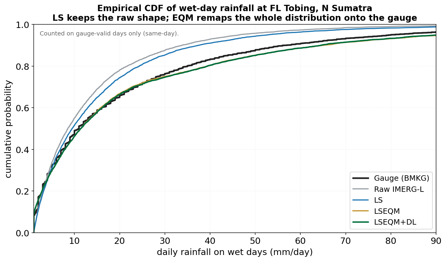
The effect is visible in the wet-day CDF below: Linear Scaling shifts the mean but keeps the shape of the raw IMERG distribution (the blue curve still bends like the grey one). EQM remaps the whole distribution onto the gauge, so the LSEQM and LSEQM+DL curves sit almost on top of the BMKG reference.
Why a Gamma body, GPD tail
The empirical CDF is well behaved in the body of the distribution (frequent values, well sampled). It becomes unreliable above ~80th percentile, where you may only have a handful of exceedances per dekad. Two failure modes are common:
- Saturation at the highest observed quantile. An empirical CDF cannot map a value larger than the largest CPC observation; large IMERG events get clipped.
- Discrete jumps in the tail. With few exceedances, the empirical inverse CDF is a step function with visible discontinuities.
To prevent both, the body is fit with a parametric Gamma distribution (which provides a smooth interpolation) and the tail is replaced by a GPD fit above the 80th percentile. See GPD Tail.
Matching a 0.5 deg reference to a 0.1 deg product (BCSD)
CPC-UNI is gauge-interpolated at 0.5 deg, but IMERG is corrected at 0.1 deg - one CPC cell spans a 5 x 5 block of IMERG pixels. The framework does not regrid the rainfall data; instead it follows the BCSD principle (Wood et al. 2004): fit the correction parameters on the native CPC grid, then disaggregate the parameters to the fine grid.
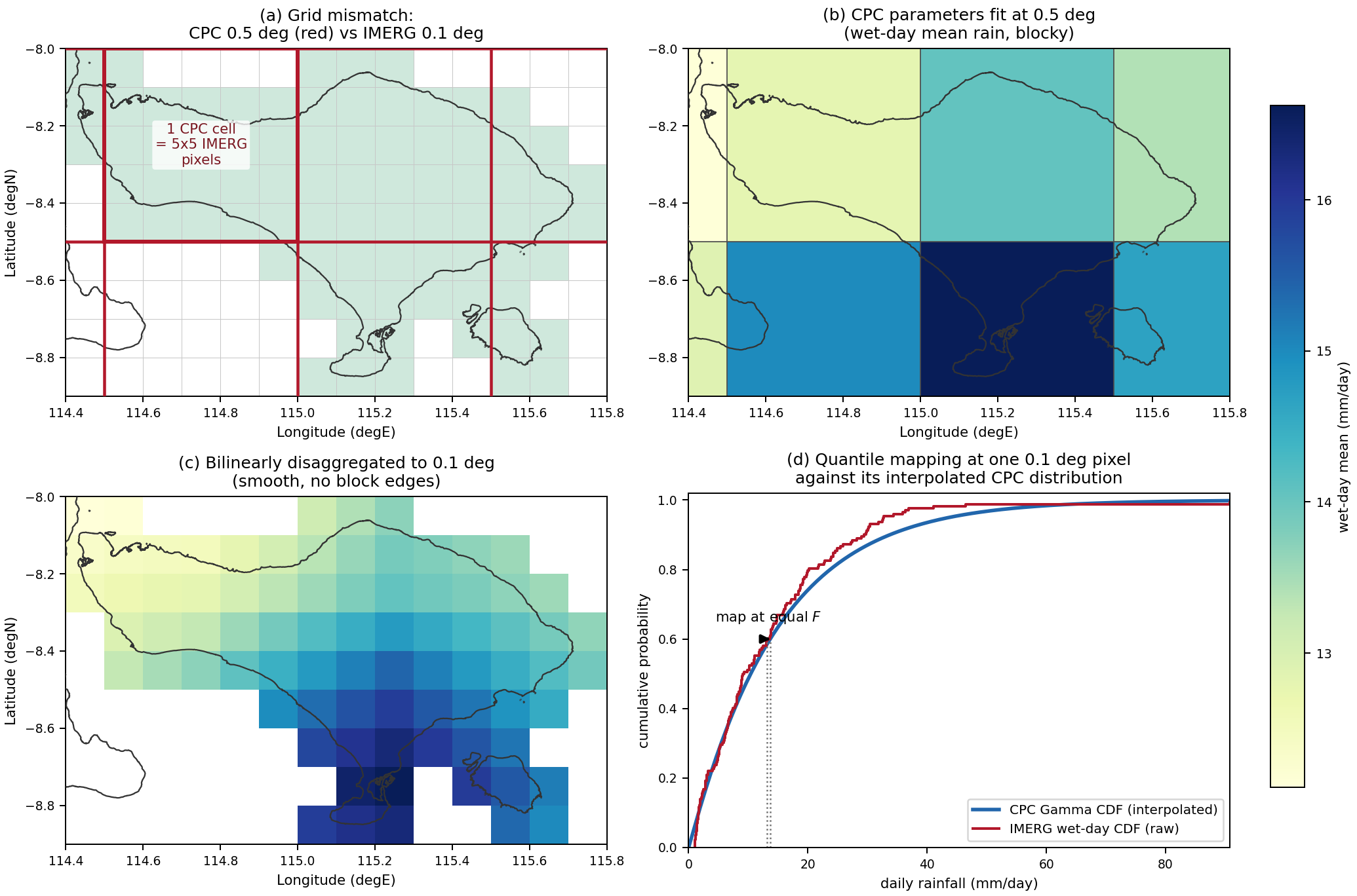
The key idea: the correction is disaggregated, not the rainfall. IMERG keeps its native 0.1 deg spatial detail; only the climatological target (the Gamma shape and scale, the GPD threshold, the dry-day fraction) is interpolated down from the coarser reference. This is what fit_cpc_parameters_on_native_grid followed by interpolate_cpc_params_to_imerg_grid does in the code - see Implementation > EQM.
Wet / dry handling
Days below the 1.0 mm wet-day threshold are treated as dry. The threshold is the value used in WMO categorical metrics and the default wet_day_threshold in config.yml. EQM handles dry days in two ways:
- A dry input stays dry. Quantile mapping is applied only to above-threshold IMERG days; the output array is zero-initialised, so a day the satellite already reports as dry comes out as exactly zero.
- Over-detected drizzle is suppressed to dry. Raw IMERG rains on too many days. EQM matches the corrected product’s dry-day fraction to the reference (Cannon 2015, §3.2): the smallest over-detected wet values, whose position in the unconditional distribution falls below the reference dry-day fraction, are set to zero.
This is a first-order property, not a corner case: dry days are about half the validated record. The effect is a clear gain in dry-day agreement. On a day the gauge records as dry, the corrected product is also dry about 69% of the time, up from ~56% before the distribution step, and the wet-day-frequency ratio moves from 1.21 (over-detecting) toward 0.95.
The same mechanism that removes false drizzle also costs a little hit rate: probability of detection drops from about 0.78 to 0.65 as the over-detected light-rain days are reclassified as dry. Fewer false alarms at the cost of some light-rain hits - not a free win. The CNN refinement stage leaves dry days untouched; this is purely the EQM stage. (Numbers from the 172-station Indonesia validation.)
Implementation
src/bias_correction.py - the lseqm() function, which calls src/distribution_fitting.py for the Gamma and GPD fits.
The full LSEQM correction (LS + EQM + GPD) is what the framework labels lseqm. The chain runs as one function call per dekad.
References
- Wood, A. W., Leung, L. R., Sridhar, V., & Lettenmaier, D. P. (2004). Hydrologic implications of dynamical and statistical approaches to downscaling climate model outputs. Climatic Change, 62(1-3), 189-216. (BCSD parameter disaggregation.)
- Cannon, A. J., Sobie, S. R., & Murdock, T. Q. (2015). Bias correction of GCM precipitation by quantile mapping: how well do methods preserve changes in quantiles and extremes? Journal of Climate, 28(17), 6938-6959. (Dry-day frequency matching, §3.2.)