CNN Refinement
After LSEQM, the marginal distribution matches CPC at each pixel. What remains is the spatial residual: where does LSEQM systematically over- or underestimate compared to the reference field, in patterns a per-pixel correction cannot see?
Architecture
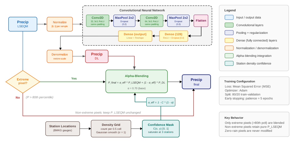
A small 2-layer convolutional network:
- Conv2D #1: 32 filters, 3 x 3 kernel, ReLU, followed by 2 x 2 max-pooling, dropout 0.2
- Conv2D #2: 64 filters, 3 x 3 kernel, ReLU, followed by 2 x 2 max-pooling, dropout 0.3
- Flatten + Dense: 128 units, ReLU, dropout 0.4
- Output: linear, one value per pixel
Trained per dekad. Input is the LSEQM-corrected field for that dekad across all years; target is the CPC field for the same days. Optimizer: Adam. Early stopping with patience 5 on a 20% validation split.
This is intentionally small. On a 0.1 deg Indonesia grid (171 x 461) the Flatten -> Dense layer already dominates the parameter count, and it grows with AOI size; going deeper would inflate it further without meaningfully improving skill for this task.
Why not a U-Net
A U-Net would skip the Flatten -> Dense bottleneck and preserve spatial dimensions throughout. It would also produce a tighter parameter budget. The current architecture predates that design choice and has been evaluated against the held-out BMKG stations; switching to U-Net is a planned improvement, tracked in the Changelog.
What the CNN actually learns
In practice the CNN learns three things:
- Coastal and orographic bias. LSEQM tends to over-smooth gradients near coasts and steep terrain; the CNN sharpens them.
- Convective extreme refinement. Heavy-rain pixels can be nudged by several percent to better match CPC’s spatial coherence on convection days.
- Diffuse-precipitation suppression. Pixels with very light precipitation that LSEQM nudges upward sometimes get pulled back down.
The amount of correction is modest by design - see Blending.
How much the CNN moves, per station
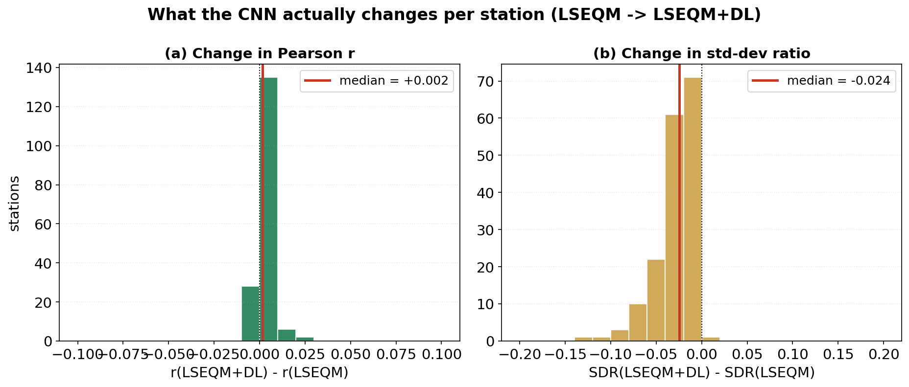
The per-station change from LSEQM to LSEQM+DL is small and centred near zero: across the validated BMKG stations the median change in daily correlation is about +0.002 and the median change in standard-deviation ratio about -0.024. The CNN tightens the variance slightly and does not degrade correlation; it is a refinement, not a second correction stage.
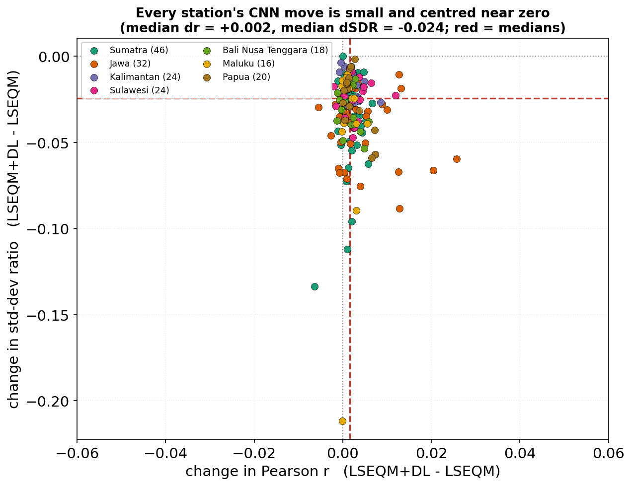
Plotting the two changes jointly, coloured by region, shows the same point from a different angle: the cloud sits tight around the origin, and the stations that move furthest are the Jawa sites - exactly where the gauge network is densest and the confidence mask opens the CNN up. Everywhere else the move is barely distinguishable from zero.
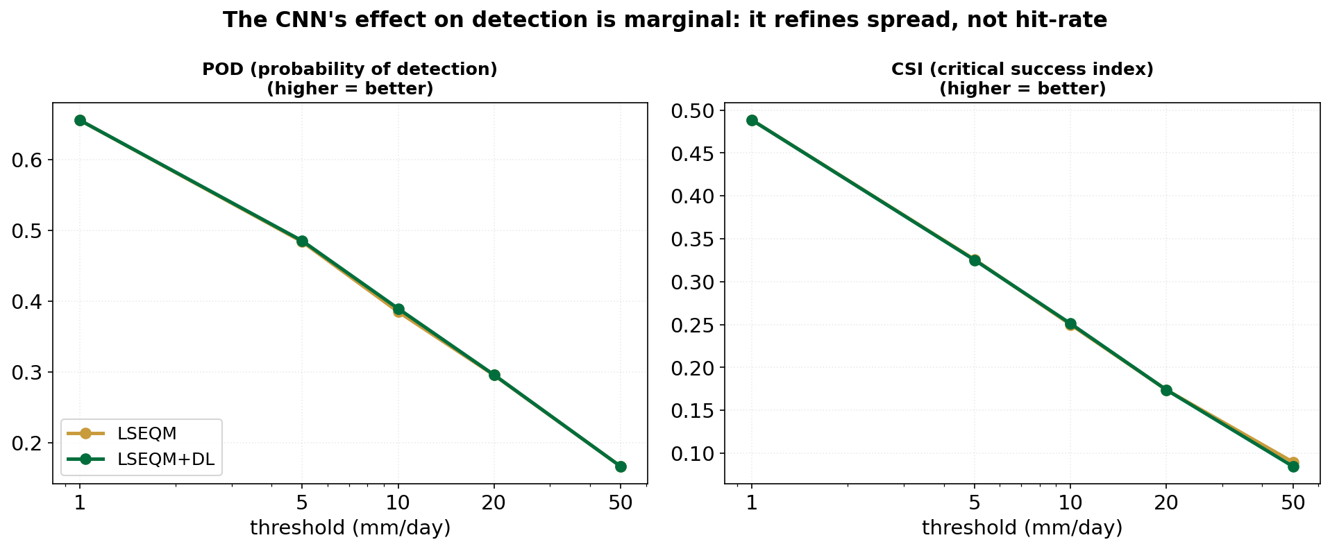
The same restraint shows up in categorical detection. Plotting POD and CSI against intensity threshold, the LSEQM and LSEQM+DL curves sit on top of each other: the CNN refines spread and tail shape, but it does not change when the product says it rains. Detection skill is set earlier in the chain and the CNN leaves it untouched.
This modest footprint is the intended behaviour. The deep-learning stage is gated by station density (see Confidence Mask), so it only acts where gauge support justifies it, and the statistical core (LSEQM) remains the physical floor everywhere else.
Implementation
src/deep_learning.py - train_bias_correction_model() (which builds and fits the network) and apply_deeplearning_model(). Trained models land in output/trained_models/.