GPD Tail Correction
Above the 80th percentile, the EQM correction is replaced by a Generalized Pareto Distribution (GPD) fit. This handles the extreme part of the distribution where empirical sampling is too sparse to be reliable.
The GPD
For exceedances \(X\) above threshold \(u\):
\[ P(X - u > x \mid X > u) = \left( 1 + \frac{\xi x}{\sigma} \right)^{-1/\xi} \]
with shape \(\xi\) and scale \(\sigma\). The shape parameter governs the heaviness of the tail: \(\xi > 0\) means a heavier-than-exponential tail (typical for tropical convection), \(\xi = 0\) is exponential, \(\xi < 0\) is bounded.
What the tail graft fixes
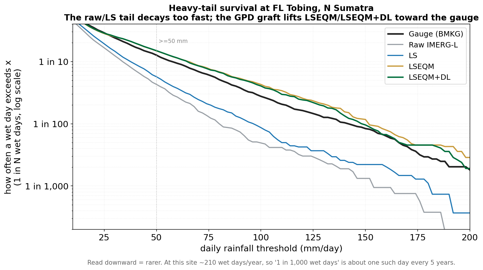
Raw IMERG and LS decay too fast in the tail: heavy days that the gauge records once every few years are systematically under-represented. The survival curve below (how often a wet day exceeds a given threshold, log scale) shows the raw and LS curves dropping away from the gauge, while the GPD graft lifts LSEQM / LSEQM+DL back toward the BMKG reference at the high-intensity end.
Fitting protocol
- Threshold: 80th percentile of the CPC wet-day values for the dekad (days above
wet_day_threshold), configurable viagpd_threshold_percentile. - Stability: Fit is K-Fold cross-validated (default K=5) and the mean shape and scale are used. This reduces the variance of the estimate when exceedances are few.
- Upper cap: After mapping, values are capped at the 99.9th percentile of the CPC reference (configurable via
upper_cap_threshold_percentile) to avoid physically unrealistic extrapolation.
Sensitivity caveats
The 80th percentile threshold is a convention from precipitation extreme-value literature, not the result of a formal optimization on this dataset. A lower threshold (e.g., 75th) yields more data for the GPD fit but blurs the boundary between the gamma body and the GPD tail. A higher threshold (e.g., 90th-95th) targets only the most extreme events but leaves fewer exceedances per dekad, sometimes fewer than the K-Fold split can absorb.
Sensitivity to this choice should be acknowledged when reporting results.
Implementation
src/distribution_fitting.py - fit_generalized_pareto_distribution() and cross_validate_gpd(), called from fit_cpc_parameters_on_native_grid(). The mapping is applied inside gamma_quantile_mapping_precomputed(), which runs in the EQM loop of lseqm() in src/bias_correction.py.
References
- Coles, S. (2001). An Introduction to Statistical Modeling of Extreme Values. Springer.
- Hosking, J. R. M., & Wallis, J. R. (1997). Regional Frequency Analysis: An Approach Based on L-Moments. Cambridge University Press.