viewof inputSeason = selectControl("Input season", seasonChoices, "OND")
inputSummary(fitData, inputSeason)From rainfall inputs to a calibrated forecast
Fit and diagnose OND and JJA 2023 forecasts with PyCPT
Case 02 · Model fitting and diagnostics · Full Indonesia
The first case asked whether calibrated forecasts were better than the raw model and a simple rainfall average. This case opens the fitting workflow itself. What goes into PyCPT? What does it return? And what should we learn from its model patterns before interpreting a forecast map?
We follow October–December (OND) 2023, then apply the same choices to June–August (JJA) 2023. Both cover full Indonesia. The executed notebook runs four actual PyCPT fits (CCA and PCR for each season) and checks the results against the original verified controls. All inputs are local seasonal fields.
NoteChoose how to follow along
Read this story and the executed notebook in your browser. To execute the fitting cells, use the full tested PyCPT environment with its compatible CPT engine. The smaller analysis-only environment remains suitable for the first case and for exploring exported NetCDFs. Neither local-input path requires an IRIDL key. Setup and complete fitting kit.
The interactive views below share the notebook’s computed outputs. Hover, tap or focus chart marks to inspect values. Maps support arrow keys after receiving focus. PNG downloads include the current selections; chart views also offer SVG. For the pattern explorer, SVG contains the score series and PNG contains the maps and series together. Labelled notebook-reference links retain the static figures.
Begin with three inputs
Think of the fitting call as a relationship between X, Y and F. X contains past model rainfall, Y contains observed rainfall for those same target seasons, and F contains the model forecast for the new target. The relationship learned from X and Y is applied to F.
Here X and F are CFSv2 ensemble-mean seasonal rainfall on a 1° grid. The predictor domain extends beyond Indonesia, from 85–155°E and 20°S–20°N. Y is CHIRPS3 seasonal rainfall aggregated to the existing 0.25° country-land grid. It has 3,240 complete locations used by both calibrated methods and the baselines. The finer output grid describes the aggregation and output locations; it does not establish independent dynamical predictability at 0.25°.
Training uses 30 annual seasonal samples from 1991–2020. The 2023 predictor is separate: OND starts from the September initialization, while JJA starts from May. The notebook checks the actual target bounds, matching X/Y years, units and complete support before calling PyCPT. The kit begins with prepared seasonal totals in millimetres; the source and preprocessing hashes accompany those files.
Fit a controlled comparison
The notebook uses PyCPT’s direct fitting interface, demonstrated in the official core example. CCA and PCR both retain three predictor EOFs. CCA also retains three predictand EOFs and two CCA modes. These counts stay fixed between OND and JJA. They make the comparison reproducible; they have not been shown to be optimal.
Both fits use CPT’s five-sample cross-validation window. For each training target, the calculation omits that sample and two neighbours on either side, wrapping at the ends of the training sequence. It refits the model for that hindcast. The separate 2023 forecast is then made with the final model fitted to all 30 training seasons. The IRI validation reference introduces the distinction between validation and the fitted regression model.
CCA returns five datasets: hindcasts, forecasts, native skill, X patterns and Y patterns. PCR returns four, with X patterns and no Y pattern decomposition. The notebook retains every dataset and writes additional cleaned diagnostics. Each fit has its own directory, command record, log and numerical control checks. There are no source downloads or fitted-probability scoring steps in this lesson.
TipStart with the forecast result, then inspect the model
OND 2023: national spatial RMSE was 292.39 mm for raw CFSv2, 226.50 mm for climatology, 120.35 mm for CCA and 117.36 mm for PCR.
JJA 2023: national spatial RMSE was 377.82 mm for raw CFSv2, 130.69 mm for climatology, 177.98 mm for CCA and 175.59 mm for PCR.
Notebook reference PNG · all three forecast metrics and both seasons
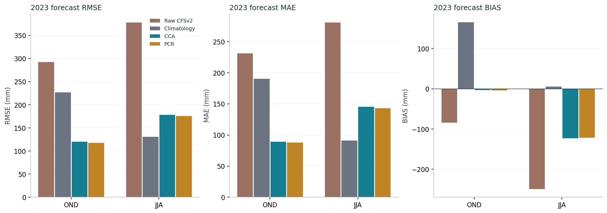
RMSE and MAE measure spatial rainfall errors over the shared land cells. Bias is forecast minus observed rainfall: negative means too little rain. The score is not the error of a single national-average rainfall estimate. The sample selector keeps the 2023 comparison separate from pooled training CV diagnostics; these cover different years and answer different questions.
What was compressed?
An EOF represents a pattern of variation in a training field. Its score describes how that pattern varies through the training years. PCR uses a small collection of predictor scores in its regression. CCA first compresses both the predictor and predictand fields, then relates their component combinations.
A scree plot shows how much training-field variance each EOF accounts for. The complete spectrum here has 30 entries, while the model retains only the first three. A larger retained percentage is a statement about compression. It is not a percentage of correctly forecast rainfall or a forecast-skill score. The official scree-plot reference describes the variance interpretation.
Notebook reference PNG · X/Y spectra for both seasons
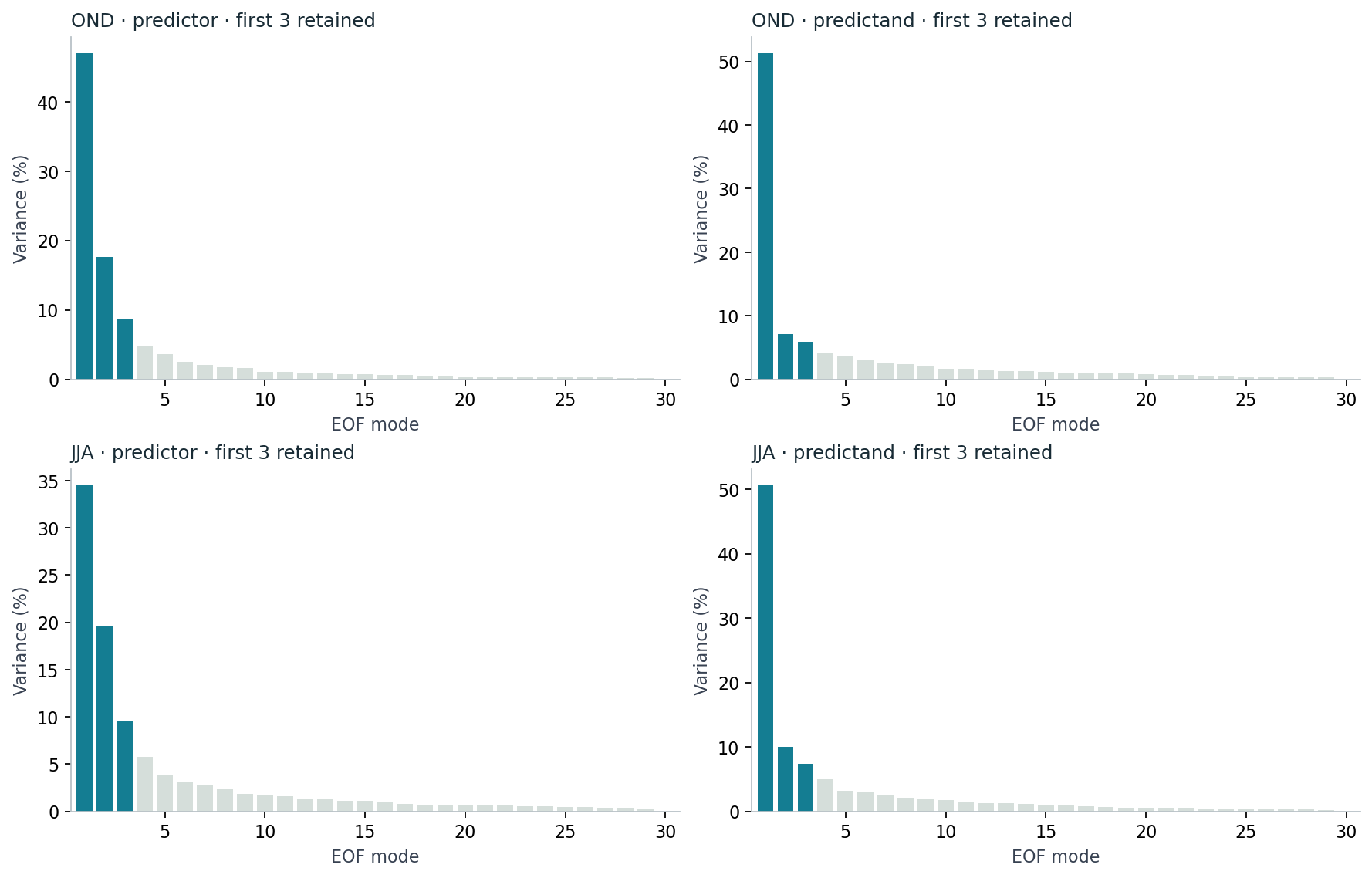
In these controlled fits, the saved predictor EOF files are identical between CCA and PCR for each season. They start with the same predictor compression. Their later regression construction differs. We keep the first three modes throughout this lesson rather than searching for a more flattering 2023 result.
Read patterns alongside their time series
CCA constructs pairs of predictor and predictand component series whose training correlation is maximized within the retained spaces. The maps below show how each original rainfall field relates to its own saved score. The score lines are standardized separately so their variations can be viewed together.
These are field–score correlations calculated from the training data. Native exported weights have a different meaning; the EOF output reference and CCA reference distinguish saved weights from displayed correlations. The notebook verifies missing-value masks and exports the two quantities under separate names.
Notebook reference PNG · OND CCA pair 1 · JJA CCA pair 1
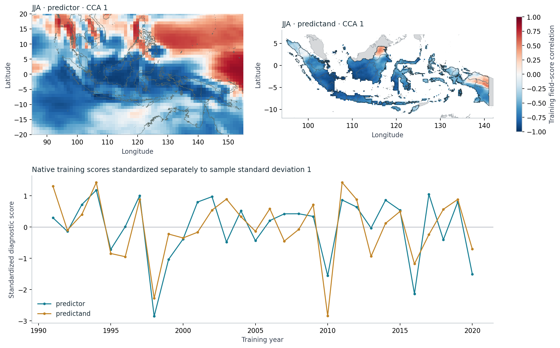
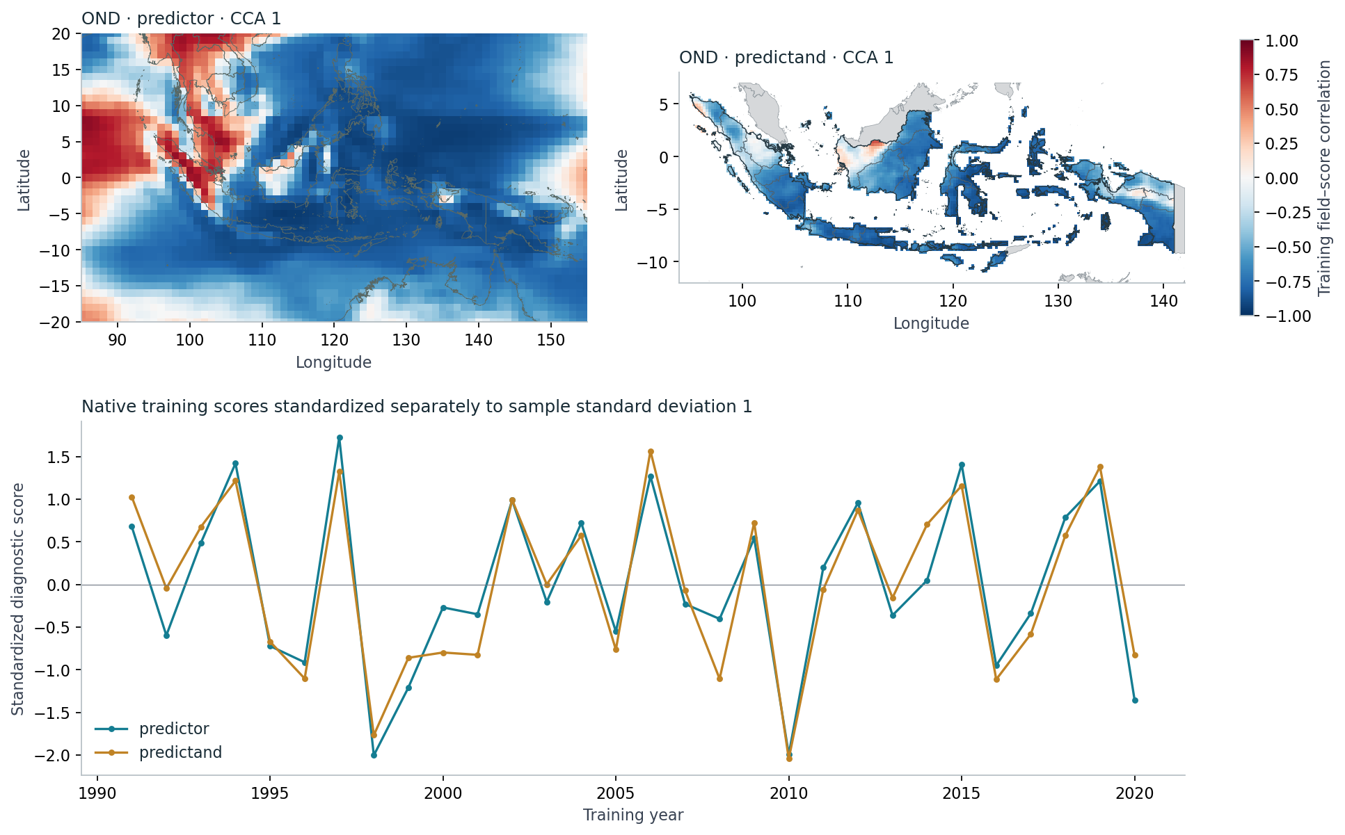
The X map includes the whole predictor domain, including ocean model rainfall. The Y map shows Indonesia’s evaluated land support, with neighbouring countries grey and country/province boundaries outlined. A blank cell is outside that support, not an observed zero. The colours describe training associations, not 2023 rainfall anomalies. An EOF and its score can change sign together without changing their product; independently numbered X/Y EOFs are not canonical pairs.
ImportantCanonical correlation is a training diagnostic
A high correlation between CCA score series does not establish a good forecast. It depends partly on retained dimensions, as the official CCA guidance explains. Full-training patterns are also distinct from the EOFs rebuilt inside each CV fold. We do not infer a climate mechanism, empirical probability reliability or optimized settings from these maps. A small absolute EOF-scale discrepancy in an independent recomputation (a working record, not published) remains unresolved, so amplitude reconstruction is outside this lesson; correlation maps and variance percentages are checked separately.
Ask what the withheld years reveal
The CV residuals test deterministic predictions inside the training interval. The calibrated model excludes the five-sample window for each target. The climatology baseline below excludes the same five observations; the raw model is left uncalibrated. A simple average of all 30 observations would not be that withheld-target climatology baseline.
Notebook reference PNG · CV-year RMSE for both seasons
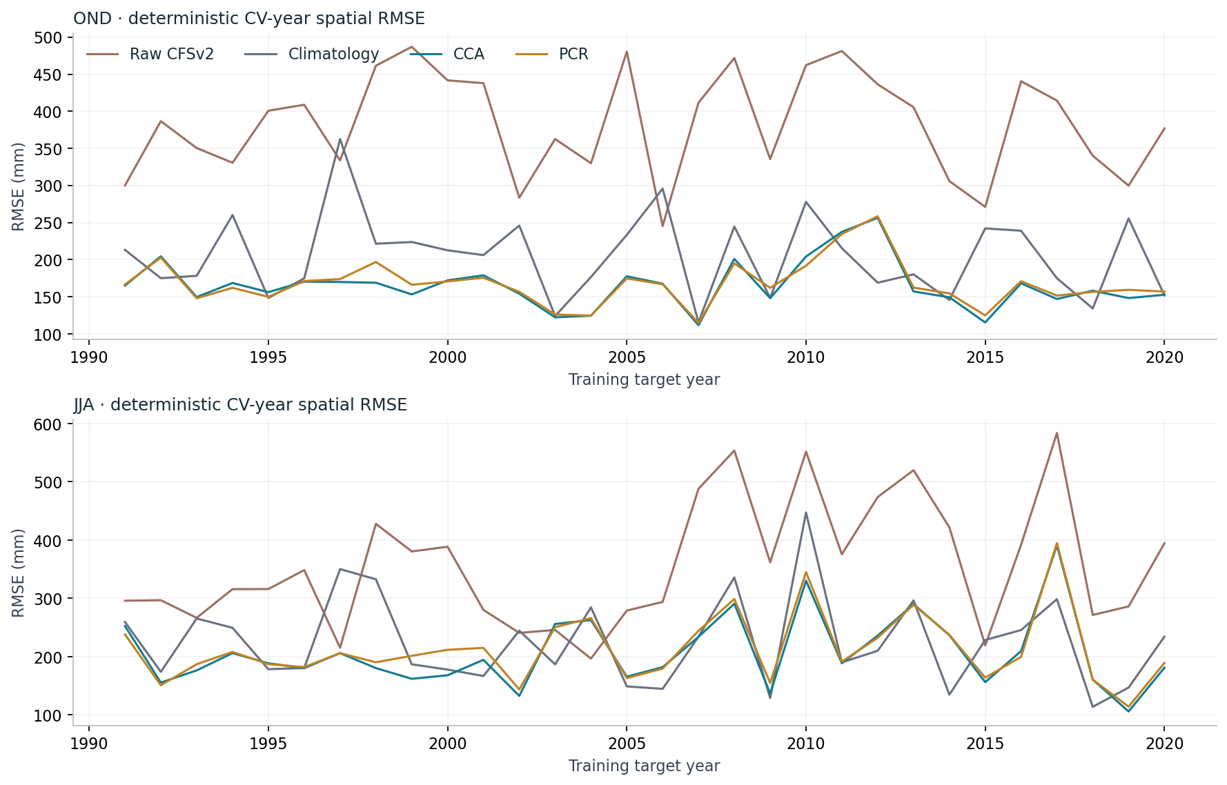
Some years are harder than others. Pooled CV RMSE takes the square root after averaging annual spatial squared errors; it is not an average of annual RMSE. Mean bias can cancel across years, and the balanced cyclic climatology mean can have essentially zero pooled bias while still making substantial errors. Keep the annual series visible alongside any pooled score.
These diagnostics also have limits. Repeated model selection against CV results can introduce selection bias. The input archive mixes reforecasts and an operational append from April 2011, so temporal completeness does not prove homogeneity. The methods guide explains the archive and validation context. No settings are tuned within this worked example.
Return to JJA with a baseline in view
The four new fits reproduce the original controls, including the JJA outcome. Both calibrations improve on the raw model’s national 2023 error in this season, while climatology has lower error than either calibrated method. A successful software run and a coherent training pattern therefore still need a forecast comparison against a simple alternative.
Notebook reference PNG · absolute errors for climatology/CCA/PCR, both seasons
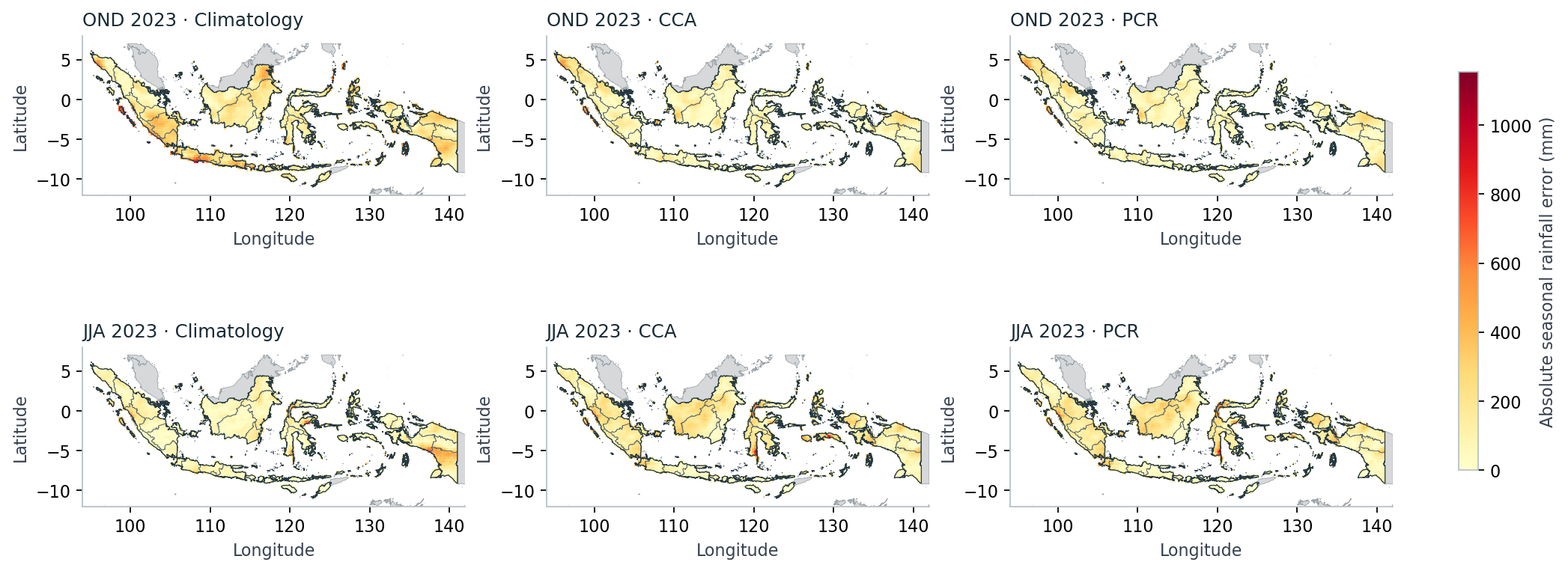
All maps within a selected view share their colour scale. Signed errors identify too-wet and too-dry predictions; absolute errors show magnitude. The two selected seasons do not establish a general relationship between canonical correlation and forecast error. Explaining the physical cause of the JJA residuals requires additional evidence beyond this fitting exercise.
Take the workflow with you
The executed companion contains the actual four fitting calls, visible score formulas, control checks and six reference figures. The complete fitting kit includes the local inputs, frozen controls, helper code, executed notebook and tested Linux environment lock. Each execution uses a new scratch directory.
- 2023 forecasts, observations and cell errors (NetCDF)
- Separate forecast/CV national scores (NetCDF) · CSV
- CV-year scores (NetCDF) · CV residual fields
- Complete fitted output archive: all 30 NetCDFs
- Control checks (CSV) · Execution and source/output manifest
- Setup and reproduction
This remains a retrospective learning case with fixed settings and deliberately selected outcomes. It establishes a reproducible fitting workflow, not general operational performance, physical attribution or calibrated probability frequencies.
References
- IRI. Guide to PyCPT 2 for Seasonal Climate Forecasts (Jupyter Book, 2 September 2023 build): The Climate Predictability Tool (CPT). https://iri.columbia.edu/~awr/pycpt/seasonal-jupyterbook/html_2sep2023/cpt.html
- IRI. CPT-Core demonstration notebook (
Demo/cptcore_demo.ipynb). iri-pycpt/notebooks, commit 1c97531. https://github.com/iri-pycpt/notebooks/blob/1c975316910b9e047ce685d9b8cdefb2c4b73551/Demo/cptcore_demo.ipynb - CPT+. 444: CCA Maps (CPT help). https://cptplus.org/Help/Tools_Models_CCA.html Same page name as on the former cpthelp.iri.columbia.edu, which did not resolve when checked on 10 November 2026.
- CPT+. 441: Scree Plots (CPT help). https://cptplus.org/Help/Tools_Models_Scree.html Same page name as on the former cpthelp.iri.columbia.edu, which did not resolve when checked on 10 November 2026.
- CPT+. 443: Y Loadings and Scores (CPT help). https://cptplus.org/Help/Tools_Models_YEOF.html Same page name as on the former cpthelp.iri.columbia.edu, which did not resolve when checked on 10 November 2026.
- IRI. CPT+: Climate Predictability Tool. https://iri.columbia.edu/our-expertise/climate/tools/cpt/
- IRI Data Library. NMME NCEP-CFSv2 hindcasts, PENTAD_SAMPLES_FULL, precipitation. https://iridl.ldeo.columbia.edu/SOURCES/.Models/.NMME/.NCEP-CFSv2/.HINDCAST/.PENTAD_SAMPLES_FULL/.prec/ Browsing Data Library pages requires signing in (checked 10 November 2026); PyCPT’s data requests in this tutorial succeeded without a key.
- Saha, S., Moorthi, S., Wu, X., et al. (2014). The NCEP Climate Forecast System Version 2. Journal of Climate, 27(6), 2185-2208. https://doi.org/10.1175/JCLI-D-12-00823.1
- Kirtman, B., Min, D., Infanti, J., et al. (2014). The North American Multimodel Ensemble: Phase-1 seasonal-to-interannual prediction; Phase-2 toward developing intraseasonal prediction. Bulletin of the American Meteorological Society, 95(4), 585-601. https://doi.org/10.1175/BAMS-D-12-00050.1
- Climate Hazards Center, UC Santa Barbara. CHIRPS: Rainfall Estimates from Rain Gauge and Satellite Observations (CHIRPS version 3.0 page). https://www.chc.ucsb.edu/data/chirps3
- Funk, C., Peterson, P., Landsfeld, M., et al. (2014). A quasi-global precipitation time series for drought monitoring. U.S. Geological Survey Data Series 832. https://doi.org/10.3133/ds832