Evaluate a model

Fit CCA with evaluate_models, read what it returns, and check it

evaluate_models is the step that calls CPT. It fits the calibration, produces cross-validated hindcasts, a forecast for 2023 and skill maps, and writes them to the case folder. This chapter runs it on the inputs from chapters 2 and 3, then looks closely at what each returned number is, because the returned objects mix results of different kinds.

What you need to run this page

The full PyCPT environment with its CPT engine, and the case folder from chapters 1 to 3. No data is downloaded: PyCPT reuses the files already in the folder.

1. Load the inputs

The settings are the ones from chapter 1. The predictor files come from chapter 2 and the predictand is the local CHIRPS v3.0 file built in chapter 3.

from pathlib import Path
import datetime as dt
import inspect
import sys
import time

import matplotlib.pyplot as plt
import numpy as np
import pandas as pd
import xarray as xr
from IPython.display import Image, display
import pycpt
from pycpt import notebook as pycpt_notebook

repo = next((p for p in (Path.cwd(), *Path.cwd().parents) if (p / "pycpt_tutorial").is_dir()), None)
sys.path.insert(0, str(repo))
from pycpt_tutorial import figures
figures.use_style()

MOS = "CCA"
predictor_names = ["CFSv2.PRCP"]
predictand_name = "CHIRPS3.PRCP"
download_args = {
    "fdate": dt.datetime(2023, 9, 1),
    "target": "Oct-Dec",
    "target_first_year": 1991,
    "target_final_year": 2020,
    "predictor_extent": {"west": 85, "east": 155, "south": -20, "north": 20},
    "predictand_extent": {"west": 94, "east": 142, "south": -12, "north": 7},
}
cpt_args = {
    "transform_predictand": None,
    "tailoring": None,
    "cca_modes": (2, 2),
    "x_eof_modes": (3, 3),
    "y_eof_modes": (3, 3),
    "validation": "crossvalidation",
    "drymask_threshold": None,
    "skillmask_threshold": None,
    "crossvalidation_window": 5,
    "synchronous_predictors": True,
}
force_download = False

case_dir = Path.home() / "PyCPT" / "indonesia-ond-2023-sep-init"
domain_dir = pycpt.setup(case_dir, download_args["predictor_extent"])
local_predictand_file = domain_dir / "data" / "local-CHIRPS3-OND-1991-2020.nc"
Y, hindcast_data, forecast_data = pycpt.download_data(
    predictand_name, local_predictand_file, predictor_names,
    download_args, domain_dir, force_download)

Input data will be saved in ~/PyCPT/indonesia-ond-2023-sep-init/85W-155E_to_-20S-20N/data
Figures will be saved in ~/PyCPT/indonesia-ond-2023-sep-init/85W-155E_to_-20S-20N/figures
Output will be saved in ~/PyCPT/indonesia-ond-2023-sep-init/85W-155E_to_-20S-20N/output
Reusing already-downloaded CFSv2.PRCP_f2023

Using local observed predictand dataset
Reusing already-downloaded CFSv2.PRCP

The predictand is named CHIRPS3.PRCP here, not CHIRPS3 (local) as in chapter 3. For a local file the name is only a label, but step 7 shows that one plotting function reads it.

2. What `evaluate_models` does

Before running it, read it. For CCA, the installed PyCPT 2.10.4 source does the following for each model:

source = inspect.getsource(pycpt_notebook.evaluate_models).splitlines()
start = next(i for i, line in enumerate(source) if "if str(MOS).upper() == 'CCA'" in line)
end = next(i for i, line in enumerate(source) if "elif str(MOS).upper() == 'PCR'" in line)
for number in range(start, end):
    if source[number].strip():
        print(f"{number + 1:4d} | {source[number]}")

  24 |         if str(MOS).upper() == 'CCA':
  26 |             # fit CCA model between X & Y and produce real-time forecasts for F
  27 |             cca_h, cca_rtf, cca_s, cca_px, cca_py = cc.canonical_correlation_analysis(
  28 |                 model_hcst, Y, F=forecast_data[i], **cpt_args
  29 |             )
  31 |             # fit CCA model again between X & Y, and produce in-sample probabilistic hindcasts
  32 |             # this is using X in place of F, with the year coordinates changed to n+100 years
  33 |             # because CPT does not allow you to make forecasts for in-sample data
  34 |             cca_h, cca_f, cca_s, cca_px, cca_py = cc.canonical_correlation_analysis(
  35 |                 model_hcst, Y, \
  36 |                 F=ce.redate(model_hcst, yeardelta=48), **cpt_args
  37 |             )
  38 |             cca_h = xr.merge([cca_h, ce.redate(cca_f.probabilistic, yeardelta=-48), ce.redate(cca_f.prediction_error_variance, yeardelta=-48)])
  40 |             # use the in-sample probabilistic hindcasts to perform probabilistic forecast verification
  41 |             # warning - this produces unrealistically optimistic values
  42 |             cca_pfv = cc.probabilistic_forecast_verification(cca_h.probabilistic, Y, **cpt_args)
  43 |             cca_s = xr.merge([cca_s, cca_pfv])
  45 |             hcsts.append(cca_h)
  46 |             fcsts.append(cca_rtf)
  47 |             skill.append(cca_s.where(cca_s > -999, other=np.nan))
  48 |             pxs.append(cca_px)
  49 |             pys.append(cca_py)

Read it as three steps:

First fit. CCA on X and Y with F set to the real 2023 forecast input. Only the forecast from this call (cca_rtf) is kept.
Second fit. The same CCA again, but F is the training predictor X itself, shifted forward by 48 years with cptextras.redate so CPT will accept it as “future” input. (The comment above the call says 100 years; the code passes yeardelta=48.) The probabilities and prediction-error variance from this call are shifted back and merged into the hindcasts. They are probabilities for years the model was trained on.
Probabilistic scores are computed from those in-sample probabilities. The source’s own comment says this “produces unrealistically optimistic values”.

The second call also replaces the first call’s hindcasts, skill and patterns. Its cross-validation uses the same X, Y and settings as the first.

3. Run it

start = time.monotonic()
hcsts, fcsts, skill, pxs, pys = pycpt.evaluate_models(
    hindcast_data, MOS, Y, forecast_data, cpt_args, domain_dir, predictor_names)
print(f"evaluate_models finished in {time.monotonic() - start:.0f} s")

evaluate_models finished in 38 s

4. What came back

Five lists, one entry per model. With one model, each list has one item.

rows = []
for name, ds in [("hcsts", hcsts[0]), ("fcsts", fcsts[0]), ("skill", skill[0]),
                 ("pxs", pxs[0]), ("pys", pys[0])]:
    for variable, a in ds.data_vars.items():
        rows.append({"returned": name, "variable": variable,
                     "dimensions": ", ".join(f"{d}={n}" for d, n in a.sizes.items()),
                     "units attribute": a.attrs.get("units", "")})
pd.DataFrame(rows)

	returned	variable	dimensions	units attribute
0	hcsts	deterministic	T=30, Y=76, X=192	mm
1	hcsts	probabilistic	C=3, T=30, Y=76, X=192	probability (%)
2	hcsts	prediction_error_variance	T=30, Y=76, X=192	mm (squared)
3	fcsts	deterministic	T=1, Y=76, X=192	mm
4	fcsts	probabilistic	C=3, T=1, Y=76, X=192	probability (%)
5	fcsts	prediction_error_variance	T=1, Y=76, X=192	mm (squared)
6	skill	pearson	Y=76, X=192
7	skill	spearman	Y=76, X=192
8	skill	two_alternative_forced_choice	Y=76, X=192
9	skill	roc_area_below_normal	Y=76, X=192
10	skill	roc_area_above_normal	Y=76, X=192
11	skill	root_mean_squared_error	Y=76, X=192
12	skill	generalized_roc	Y=76, X=192
13	skill	ignorance	Y=76, X=192
14	skill	rank_probability_skill_score	Y=76, X=192
15	pxs	x_cca_scores	T=30, Mode=30
16	pxs	x_eof_scores	T=30, Mode=30
17	pxs	x_cca_loadings	Mode=30, Y=41, X=71
18	pxs	x_eof_loadings	Mode=30, Y=41, X=71
19	pxs	x_explained_variance	Mode=30
20	pys	y_cca_scores	T=30, Mode=30
21	pys	y_eof_scores	T=30, Mode=30
22	pys	y_cca_loadings	Mode=30, Y=76, X=192
23	pys	y_eof_loadings	Mode=30, Y=76, X=192
24	pys	y_explained_variance	Mode=30

print("Files written to output/:")
for f in sorted((domain_dir / "output").iterdir()):
    print(f"  {f.name}  ({f.stat().st_size / 1000:.0f} kB)")

Files written to output/:
  CFSv2.PRCP_cca_x_spatial_loadings.nc  (1437 kB)
  CFSv2.PRCP_cca_y_spatial_loadings.nc  (7046 kB)
  CFSv2.PRCP_crossvalidated_cca_hindcasts.nc  (17535 kB)
  CFSv2.PRCP_realtime_cca_forecasts.nc  (607 kB)
  CFSv2.PRCP_skillscores_cca.nc  (1068 kB)

5. Which numbers are which

The step 2 source decides how each result may be used. The table summarises it.

Result	Where it comes from	Use it as
`hcsts.deterministic`	cross-validated hindcasts, window of 5	an out-of-sample check of the deterministic forecast, within the training period
`hcsts.probabilistic`, `hcsts.prediction_error_variance`	second fit, X re-dated as forecast input	in-sample: not evidence of probability skill
`fcsts` (all three variables)	first fit, the real September 2023 input	the 2023 forecast
`skill`: `pearson`, `spearman`, `two_alternative_forced_choice`, `roc_area_below_normal`, `roc_area_above_normal`, `root_mean_squared_error`	CPT’s deterministic scores; the next cell checks that they score the cross-validated hindcasts	deterministic skill, the six metrics the template plots
`skill`: `generalized_roc`, `ignorance`, `rank_probability_skill_score`	`probabilistic_forecast_verification` on the in-sample probabilities	optimistic: the template labels `generalized_roc` and `rank_probability_skill_score` “in sample”; `ignorance` comes from the same call
`pxs`, `pys`	patterns from the full training period	diagnostics, not skill

The template plots the six deterministic metrics. Chapter 5 returns to the probabilities.

The claim that the deterministic scores describe the cross-validated hindcasts can be checked directly: recompute the Pearson correlation and the RMSE between hcsts.deterministic and the observations at every cell, and compare them with CPT’s maps.

cv = hcsts[0].deterministic.transpose("T", "Y", "X")
obs = Y.transpose("T", "Y", "X")
anom_cv, anom_obs = cv - cv.mean("T"), obs - obs.mean("T")
pearson_check = (anom_cv * anom_obs).sum("T") / np.sqrt((anom_cv ** 2).sum("T") * (anom_obs ** 2).sum("T"))
rmse_check = np.sqrt(((cv - obs) ** 2).mean("T"))

for label, mine, cpt in [("pearson", pearson_check, skill[0].pearson),
                         ("root_mean_squared_error", rmse_check, skill[0].root_mean_squared_error)]:
    gap = np.abs(mine.values - cpt.transpose("Y", "X").values)
    print(f"{label}: largest difference from CPT's map {np.nanmax(gap):.4f} "
          f"over {int(np.isfinite(gap).sum())} cells")

pearson: largest difference from CPT's map 0.0000 over 3240 cells
root_mean_squared_error: largest difference from CPT's map 0.0013 over 3240 cells

6. Compare with the Fit & diagnose case

The Fit & diagnose case ran the same CCA settings through cptcore directly. Chapter 3 showed the predictand is identical. Chapter 2 showed the predictor is not: PyCPT’s CFSv2 totals weight the three months equally, while the case weighted them by days, with differences up to 8.25 mm. The table measures how much that changes the results, over the 3,240 predictand cells.

controls = repo / "docs/data/fitting-2023/controls"
control_forecast = xr.open_dataset(controls / "OND-cca-forecasts.nc")
control_hindcast = xr.open_dataset(controls / "OND-cca-hindcasts.nc")
control_skill = xr.open_dataset(controls / "OND-cca-native_skill.nc")
cells = Y.notnull().all("T")


def compare(label, ours, theirs):
    ours = ours.reindex(X=theirs["X"], Y=theirs["Y"], method="nearest", tolerance=1e-3).where(cells)
    a = ours.transpose(*theirs.dims).values
    b = theirs.values
    gap = np.abs(a - b)
    return {"result": label, "units": theirs.attrs.get("units", ""),
            "largest difference": float(np.nanmax(gap)),
            "mean difference": float(np.nanmean(gap)),
            "median of the case's values": float(np.nanmedian(np.abs(b)))}


rows = [compare(f"2023 forecast: {v}", fcsts[0][v], control_forecast[v]) for v in control_forecast.data_vars]
rows.append(compare("CV hindcasts: deterministic", hcsts[0].deterministic, control_hindcast.deterministic))
rows += [compare(f"skill: {v}", skill[0][v], control_skill[v]) for v in control_skill.data_vars]
pd.DataFrame(rows).set_index("result").round(4)

	units	largest difference	mean difference	median of the case's values
result
2023 forecast: deterministic	mm	0.0235	0.0066	617.5582
2023 forecast: probabilistic	probability (%)	0.0410	0.0057	24.1579
2023 forecast: prediction_error_variance	mm (squared)	539.3447	29.2053	30431.3300
CV hindcasts: deterministic	mm	2.5542	0.2239	783.1758
skill: pearson		0.0019	0.0004	0.5883
skill: spearman		0.0227	0.0011	0.5842
skill: two_alternative_forced_choice		0.9195	0.0619	70.8046
skill: roc_area_below_normal		0.0150	0.0005	0.8150
skill: roc_area_above_normal		0.0106	0.0007	0.7350
skill: root_mean_squared_error		0.4358	0.0578	150.9366

The predictor difference measured in chapter 2 moves the results only slightly: the 2023 deterministic forecast changes by hundredths of a millimetre, the cross-validated hindcasts by up to a few millimetres, and the skill scores by small fractions of their scales. The high-level evaluate_models path and the direct cptcore path agree to the extent the inputs agree.

7. Plot the results

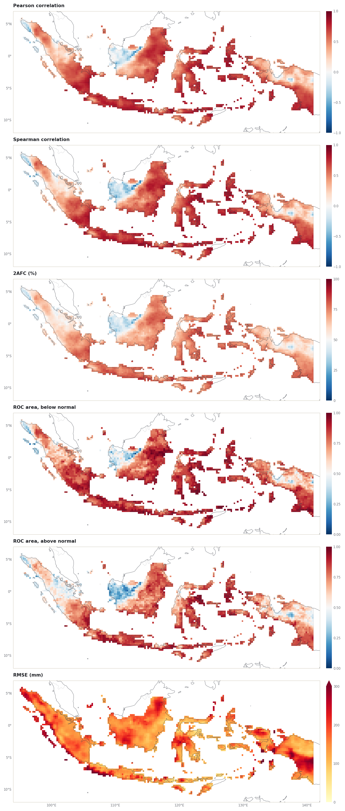
PyCPT has four plotting functions for these results: plot_skill, plot_eof_modes, plot_cca_modes and plot_forecasts. Each saves PNG files in the case’s figures/ folder. This chapter runs all four so those files exist, but draws the figures on the page with the tutorial’s figure helper from the same returned data, in one consistent style. figures.quiet_pycpt_plots() stops PyCPT from also drawing its versions inline; it does not change what PyCPT saves.

Skill maps

plot_skill takes the list of metric names to draw. These are the template’s six deterministic metrics. The colour ranges below are the ones PyCPT uses for them.

skill_metrics = ["pearson", "spearman", "two_alternative_forced_choice",
                 "roc_area_below_normal", "roc_area_above_normal", "root_mean_squared_error"]
with figures.quiet_pycpt_plots():
    pycpt.plot_skill(predictor_names, skill, MOS, domain_dir, skill_metrics)

predictor_box = figures.extent_of(download_args["predictor_extent"])
predictand_box = figures.extent_of(download_args["predictand_extent"])
figures.skill_figure(skill[0], predictand_box, skill_metrics)
plt.show()

EOF and CCA patterns

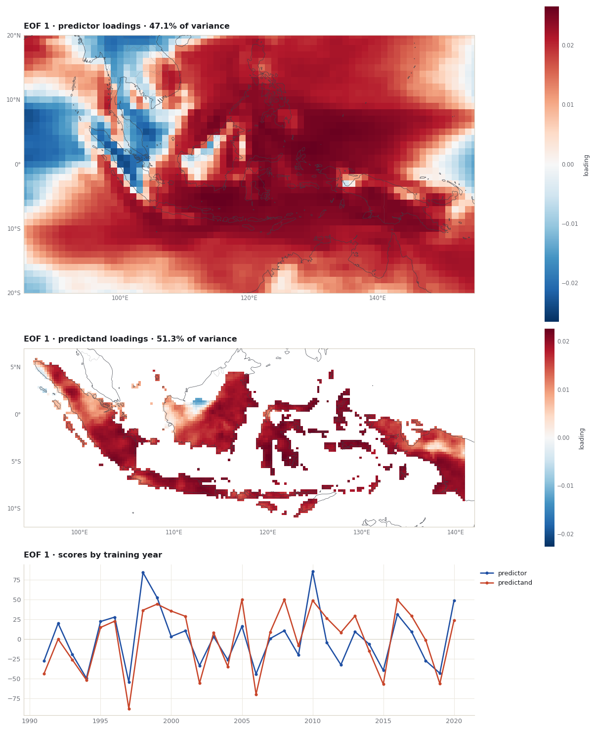
The pattern plots draw a fixed number of modes: in PyCPT 2.10.4, plot_eof_modes sets nmodes = 5 and plot_cca_modes sets nmodes = 3. This case keeps 3 EOFs and 2 CCA modes, so the cell below first checks which modes contain values.

x_patterns, y_patterns = pxs[0], pys[0]
for label, a in [("predictor EOF", x_patterns.x_eof_loadings), ("predictor CCA", x_patterns.x_cca_loadings),
                 ("predictand EOF", y_patterns.y_eof_loadings), ("predictand CCA", y_patterns.y_cca_loadings)]:
    filled = [int(m) for m in a["Mode"].values if int(a.sel(Mode=m).notnull().sum()) > 0]
    print(f"{label:>15} modes with values: {filled}")
print()
print("Predictor explained variance, modes 1-5 (%):",
      np.round(x_patterns.x_explained_variance.values[:5], 2).tolist())
print("Predictand explained variance, modes 1-5 (%):",
      np.round(y_patterns.y_explained_variance.values[:5], 2).tolist())

  predictor EOF modes with values: [1, 2, 3]
  predictor CCA modes with values: [1, 2]
 predictand EOF modes with values: [1, 2, 3]
 predictand CCA modes with values: [1, 2]

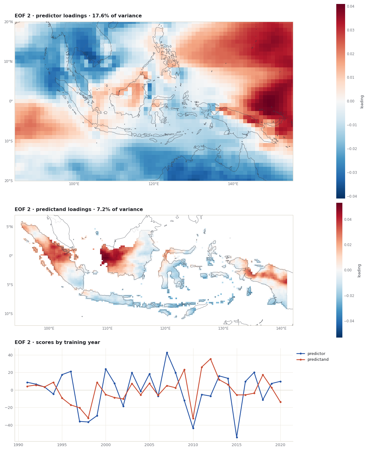
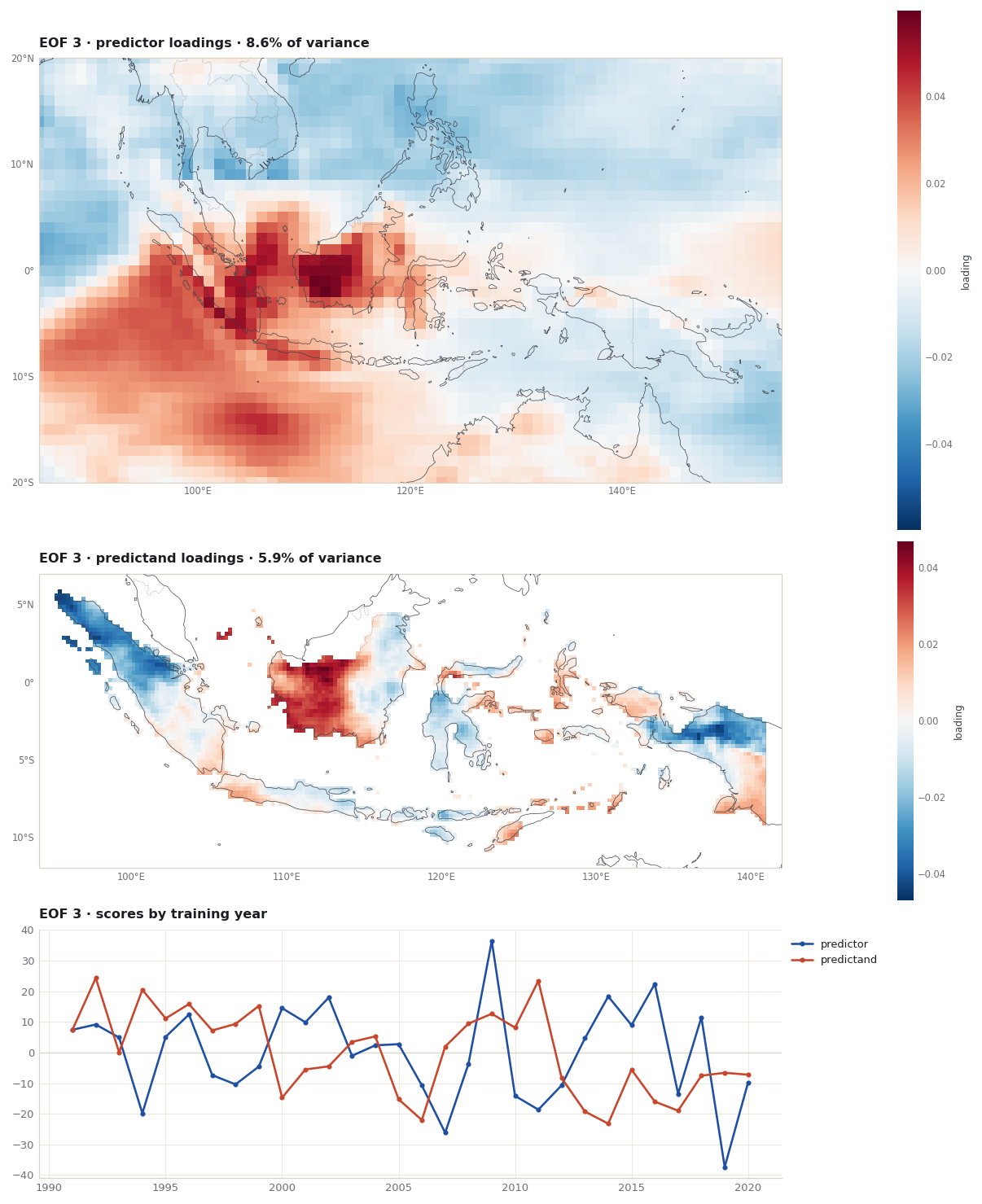
Predictor explained variance, modes 1-5 (%): [47.06, 17.62, 8.61, 4.74, 3.62]
Predictand explained variance, modes 1-5 (%): [51.33, 7.17, 5.85, 4.04, 3.61]

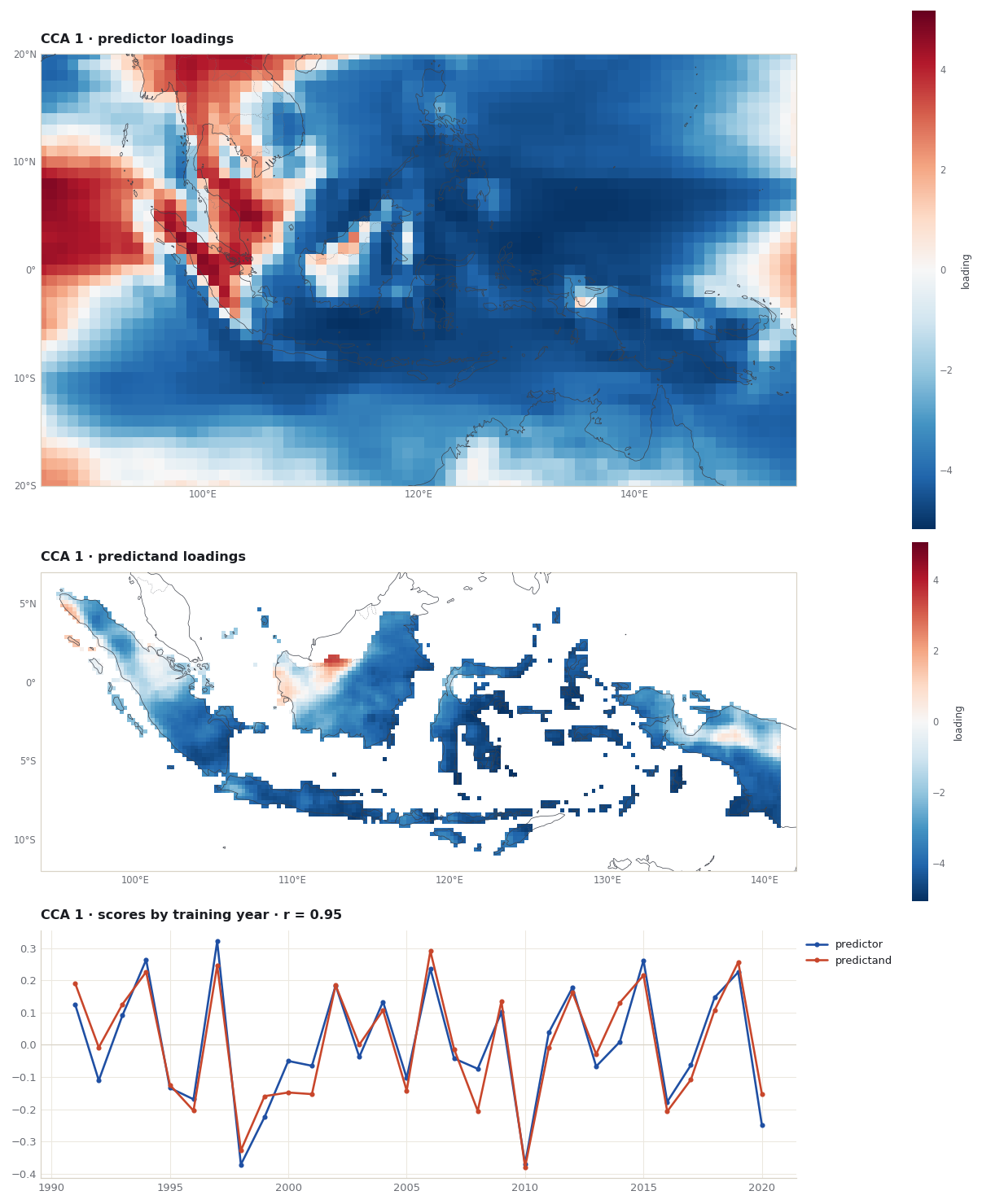
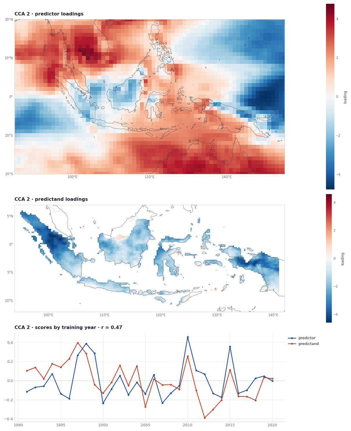
Only the retained modes have patterns; explained variance is reported for every mode, retained or not. PyCPT’s saved files therefore include empty ones: EOF modes 4 and 5, and CCA mode 3. The figures below draw the retained modes only: for each mode, the predictor loadings, the predictand loadings and the two time series of scores.

with figures.quiet_pycpt_plots():
    pycpt.plot_eof_modes(MOS, predictor_names, pxs, pys, domain_dir)
    pycpt.plot_cca_modes(MOS, predictor_names, pxs, pys, domain_dir)

for mode in [1, 2, 3]:
    figures.pattern_figure(x_patterns, y_patterns, "eof", mode, predictor_box, predictand_box)
    plt.show()

CFSV2.PRCP: EOF 1
CFSV2.PRCP: EOF 2
CFSV2.PRCP: EOF 3
CFSV2.PRCP: EOF 4
CFSV2.PRCP: EOF 5
CFSV2.PRCP: CCA MODE 1 - Canonical Correlation = 0.94
CFSV2.PRCP: CCA MODE 2 - Canonical Correlation = 0.46
CFSV2.PRCP: CCA MODE 3 - Canonical Correlation = nan

for mode in [1, 2]:
    figures.pattern_figure(x_patterns, y_patterns, "cca", mode, predictor_box, predictand_box)
    plt.show()

For CCA, the r in each title is the correlation between the predictor and predictand score series, computed in the figure from the returned scores. The sign of every mode is arbitrary: flipping both a pattern and its scores describes the same mode.

These are patterns fitted on the full training period. They show what the calibration uses; they are not evidence that the forecast is skilful.

The forecast

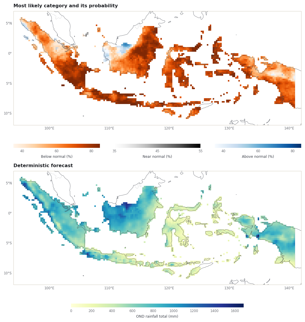
plot_forecasts chooses its colour scale by searching the predictand name for PRCP or a temperature code. In PyCPT 2.10.4, a name without one of them leaves the scale undefined and the function stops with an UnboundLocalError; with CHIRPS3 (local) as the name, it did. That is why this chapter uses CHIRPS3.PRCP.

with figures.quiet_pycpt_plots():
    pycpt.plot_forecasts(cpt_args, predictand_name, fcsts, domain_dir, predictor_names, MOS)

print("Category coordinate C:", fcsts[0].probabilistic["C"].values.tolist())
figures.forecast_figure(fcsts[0], predictand_box)
plt.show()

Category coordinate C: ['1', '2', '3']

The left map follows PyCPT’s own rule for this view (view_probabilistic in cptextras): each cell shows the category with the highest probability, coloured by that probability. Category index 0 is below normal, 1 near normal and 2 above normal, and the colour ranges, 35-85% for below and above normal and 35-55% for near normal, are the ones PyCPT uses. The right map is the deterministic forecast in mm. Chapter 5 explains how CPT defines the categories and what the probabilities mean.

print("Figures written to figures/:")
for f in sorted((domain_dir / "figures").iterdir()):
    print(f"  {f.name}")

Figures written to figures/:
  CCA_CFSv2.PRCP_CCA_mode_1.png
  CCA_CFSv2.PRCP_CCA_mode_2.png
  CCA_CFSv2.PRCP_CCA_mode_3.png
  CCA_CFSv2.PRCP_EOF_mode_1.png
  CCA_CFSv2.PRCP_EOF_mode_2.png
  CCA_CFSv2.PRCP_EOF_mode_3.png
  CCA_CFSv2.PRCP_EOF_mode_4.png
  CCA_CFSv2.PRCP_EOF_mode_5.png
  CCA_CFSv2.PRCP_[determinstic-probabilistic]-Forecast.png
  CCA_models_skillMatrices.png
  Test.png

Test.png is a working file that plot_forecasts writes and leaves behind; it is safe to ignore.

What you have now

A CCA fit through PyCPT’s own evaluate_models, with its outputs in the case folder.
A map of which returned numbers are cross-validated, which are in-sample and which are the 2023 forecast.
A measured comparison with the Fit & diagnose case: same predictand, slightly different predictor, small differences in the results.
PyCPT’s four plot functions and the files they save, with two things to watch: empty files for modes that were not retained, and the predictand name.
The same results drawn as skill maps, retained patterns and a forecast map.

The next chapter looks at the probabilistic forecast: tercile categories, CPT’s native probabilities and PyCPT’s flexible forecasts.

References

IRI. PyCPT 2.10.4 source: pycpt/src/pycpt/notebook.py (setup, download_data, summarize_available_years, evaluate_models and the plotting functions). Tag pycpt-2.10.4, commit 084bb5c. https://github.com/iri-pycpt/pycpt/blob/084bb5c380c200b5f65f11ba224a965547b91da1/pycpt/src/pycpt/notebook.py
IRI. PyCPT 2.10.4 source: pycpt/src/cptcore/functional/cca.py (canonical_correlation_analysis). Tag pycpt-2.10.4, commit 084bb5c. https://github.com/iri-pycpt/pycpt/blob/084bb5c380c200b5f65f11ba224a965547b91da1/pycpt/src/cptcore/functional/cca.py
IRI. PyCPT 2.10.4 source: pycpt/src/cptextras/redate.py (redate). Tag pycpt-2.10.4, commit 084bb5c. https://github.com/iri-pycpt/pycpt/blob/084bb5c380c200b5f65f11ba224a965547b91da1/pycpt/src/cptextras/redate.py
IRI. PyCPT 2.10.4 source: pycpt/src/cptextras/view.py (view_probabilistic) and dlcolors.py (prepare_canvas). Tag pycpt-2.10.4, commit 084bb5c. https://github.com/iri-pycpt/pycpt/blob/084bb5c380c200b5f65f11ba224a965547b91da1/pycpt/src/cptextras/view.py
IRI. PyCPT operational seasonal notebook (Operations/pycpt-operational.ipynb). iri-pycpt/notebooks, commit 1c97531. https://github.com/iri-pycpt/notebooks/blob/1c975316910b9e047ce685d9b8cdefb2c4b73551/Operations/pycpt-operational.ipynb
IRI. CPT-Core demonstration notebook (Demo/cptcore_demo.ipynb). iri-pycpt/notebooks, commit 1c97531. https://github.com/iri-pycpt/notebooks/blob/1c975316910b9e047ce685d9b8cdefb2c4b73551/Demo/cptcore_demo.ipynb
CPT+. 430: Verification (CPT help). https://cptplus.org/Help/Tools_Verify.html Same page name as on the former cpthelp.iri.columbia.edu, which did not resolve when checked on 10 November 2026.
Saha, S., Moorthi, S., Wu, X., et al. (2014). The NCEP Climate Forecast System Version 2. Journal of Climate, 27(6), 2185-2208. https://doi.org/10.1175/JCLI-D-12-00823.1
Climate Hazards Center, UC Santa Barbara. CHIRPS: Rainfall Estimates from Rain Gauge and Satellite Observations (CHIRPS version 3.0 page). https://www.chc.ucsb.edu/data/chirps3
Funk, C., Peterson, P., Landsfeld, M., et al. (2014). A quasi-global precipitation time series for drought monitoring. U.S. Geological Survey Data Series 832. https://doi.org/10.3133/ds832
Natural Earth. Admin 0: Countries, 1:10m cultural vectors. https://www.naturalearthdata.com/downloads/10m-cultural-vectors/10m-admin-0-countries/
SciTools. Cartopy (documentation). https://scitools.org.uk/cartopy/docs/latest/

1. Load the inputs

2. What evaluate_models does

3. Run it

4. What came back

5. Which numbers are which

6. Compare with the Fit & diagnose case

7. Plot the results

Skill maps

EOF and CCA patterns

The forecast

What you have now

References

2. What `evaluate_models` does