Weekly subseasonal rainfall forecasts for Indonesia at 0.05°, from GEFSv12 issued every Wednesday and calibrated with CCA and PCR through CPT
A weekly subseasonal outlook is issued on one day and covers the weeks after it. Here it is issued every Wednesday, from the GEFSv12 run started at 00 UTC that day, and gives the total rainfall of:
week 1 (days 1-7 after the issue date), week 2 (days 8-14), week 3 (days 15-21) and week 4 (days 22-28);
weeks 3-4 together (days 15-28), the period of NOAA CPC’s week 3-4 outlook.
The forecasts are calibrated with CCA and PCR through CPT against daily CHIRPS v3.0 at its native 0.05° grid, about 61,000 pixels over Indonesia, instead of the 0.25° cells of the other cases. The design (issue rule, leads, years, settings, scores) was fixed before any skill was computed.
NoteWhat you need to run this page
The full PyCPT environment with its CPT engine; daily CHIRPS v3.0 for Indonesia as yearly NetCDF files (made from the Earth Engine export by the tutorial’s gee_daily_to_netcdf.py, about 125 MB a year); and internet access the first time for about 320 GEFSv12 files from the IRI Data Library, no key needed. At 0.05° one CPT fit takes over an hour, so the ten fits run in parallel, one process each, and need about 10 free CPU cores and 25 GB of disk.
1. Issue dates, leads and training targets
GEFSv12’s hindcasts (2000-2018) start on Wednesdays, the same weekday as the issue date, so training and real time use exactly the same leads: there is no offset to bridge, unlike the dekad case. A week 5 would need model day 35, beyond the run.
The training targets are every 7-day window (14-day for weeks 3-4) that starts on a Thursday in October-December 2000-2018. For each target and lead there is exactly one Wednesday start, so all five leads are trained and scored on the same targets. 2023 follows the same rule with GEFSv12’s real-time runs. The design comes from the tutorial’s weekly GEFS download script, which the cell imports so the two cannot disagree.
from pathlib import Pathimport datetime as dtimport gzipimport jsonimport sysimport timeimport matplotlib.pyplot as pltimport numpy as npimport pandas as pdimport shapelyimport xarray as xrimport cartopy.io.shapereader as shapereaderrepo =next((p for p in (Path.cwd(), *Path.cwd().parents) if (p /"pycpt_tutorial").is_dir()), None)if repo isNone:raiseFileNotFoundError("Run this notebook inside the tutorial repository or kit.")sys.path.insert(0, str(repo))sys.path.insert(0, str(repo /"research/scripts"))from pycpt_tutorial.export import save_netcdffrom pycpt_tutorial import figuresimport download_gefs_dekads as gefs_source # request, check and download helpersimport download_gefs_weeks as weeks # the weekly designimport weekly_fits # parallel CPT fitsfigures.use_style()case_root = Path.home() /"PyCPT"/"indonesia-ond-2023-weeks"daily_dir = Path("/mnt/e/temp/chirps/daily-idn")leads =list(weeks.LEADS) # week1, week2, week3, week4, week34lead_names = weeks.LEAD_NAMEStraining_years =list(weeks.TRAINING_YEARS)settings =dict(x_eof_modes=(3, 3), validation="CROSSVALIDATION", crossvalidation_window=27, synchronous_predictors=True, transform_predictand=None, tailoring=None, drymask_threshold=None, skillmask_threshold=None)cca_settings =dict(settings, y_eof_modes=(3, 3), cca_modes=(2, 2))workers =10design = pd.DataFrame(weeks.design())for c in ["target", "end", "start"]: design[c] = pd.to_datetime(design[c])per_year = design[(design.kind =="hindcast") & (design.lead =="week1")].groupby("year").size()print(f"Training targets per year: {per_year.min()}-{per_year.max()}; "f"{design[design.kind =='hindcast'].start.nunique()} hindcast starts, "f"{design[design.kind =='forecast'].start.nunique()} real-time starts in 2023")(design.groupby(["kind", "lead"]) .agg(targets=("target", "size"), first_model_day=("first_day", "min"), days=("days", "max"), latest_model_day=("last_day", "max")) .rename(index=lead_names, level=1))
Training targets per year: 13-14; 306 hindcast starts, 16 real-time starts in 2023
targets
first_model_day
days
latest_model_day
kind
lead
forecast
Week 1
13
1
7
7
Week 2
13
8
7
14
Week 3
13
15
7
21
Weeks 3-4
13
15
14
28
Week 4
13
22
7
28
hindcast
Week 1
249
1
7
7
Week 2
249
8
7
14
Week 3
249
15
7
21
Weeks 3-4
249
15
14
28
Week 4
249
22
7
28
2. Observations: daily CHIRPS v3.0 at 0.05°
The daily files hold one field per UTC day (day D covers 00 UTC D to 00 UTC D+1), which is how GEFSv12 counts its model days too: model day d after a 00 UTC start covers the same 24 hours as observed day start + d. A target’s total is the sum of its 7 (or 14) days.
The cell after next checks that these daily values are the CHIRPS v3.0 used elsewhere in the tutorial: their sums over three dekads should equal the dekadal archive.
years =sorted(set(design.year) |set(design.year +1))files = [daily_dir /f"chirps3_rnl_daily_idn_{y}.nc"for y in years]assertall(f.exists() for f in files), [f.name for f in files ifnot f.exists()]start = time.monotonic()source = xr.open_mfdataset(files, combine="by_coords")print("Attributes:", {k: source.precip.attrs[k] for k in ("units", "long_name")})daily = source.precip.sel(time=source.time.dt.month.isin([10, 11, 12, 1])).load()print(f"Read {dict(daily.sizes)} (October-January of {years[0]}-{years[-1]}) in {time.monotonic() - start:.0f} s; "f"negative values: {int((daily <0).sum())}")
The predictand is every 0.05° pixel whose centre lies inside Indonesia (Natural Earth 1:10m), with data in all training targets. No averaging to cells: this case keeps the native grid.
records = shapereader.Reader(shapereader.natural_earth("10m", "cultural", "admin_0_countries")).records()indonesia =next(r.geometry for r in records if r.attributes["ADM0_A3"] =="IDN")shapely.prepare(indonesia)lon2d, lat2d = np.meshgrid(daily.lon, daily.lat)country = xr.DataArray(shapely.contains_xy(indonesia, lon2d, lat2d), dims=("lat", "lon"), coords={"lat": daily.lat, "lon": daily.lon})def window_totals(rows): out = []for r in rows.itertuples(): days = daily.sel(time=slice(r.target, r.end - pd.Timedelta(days=1)))assert days.sizes["time"] == r.days, (r.target, days.sizes["time"]) # every day of the window is present out.append(days.sum("time", skipna=False).assign_coords(T=r.target))return xr.concat(out, "T").rename({"lat": "Y", "lon": "X"}).sortby("Y", ascending=False)targets = {days: design[design.lead == ("week1"if days ==7else"week34")].sort_values("target").reset_index(drop=True)for days in (7, 14)}for lead in leads: # every lead uses the same target datesassert (design[design.lead == lead].sort_values("target").target.values == targets[7].target.values).all()start = time.monotonic()obs = {days: window_totals(t) for days, t in targets.items()}train = {days: (t.kind =="hindcast").values for days, t in targets.items()}mask = country.rename({"lat": "Y", "lon": "X"}).sortby("Y", ascending=False)for days in (7, 14): mask = mask & obs[days].isel(T=train[days]).notnull().all("T")print(f"Window totals built in {time.monotonic() - start:.0f} s: 7-day {dict(obs[7].sizes)}, 14-day {dict(obs[14].sizes)}")print(f"Pixels inside Indonesia: {int(country.sum()):,}; with data in every training target: {int(mask.sum()):,}")weights = np.cos(np.deg2rad(mask["Y"])) * maskdekads = xr.open_dataset("/mnt/e/temp/chirps/dekad/wld_cli_chirps3_dekad_1981_2025.nc")for first in ["2005-10-01", "2012-11-11", "2023-12-21"]: b = pd.DatetimeIndex(dekads.time_bnds.sel(time=first).values) from_daily = daily.sel(time=slice(b[0], b[1] - pd.Timedelta(days=1))).sum("time", skipna=False) stored = dekads.precip.sel(time=first).reindex(lat=daily.lat, lon=daily.lon, method="nearest", tolerance=1e-3).load() gap =abs(from_daily - stored).where(country) differ = from_daily.isnull() != stored.isnull()print(f"dekad {b[0]:%d %b %Y} ({(b[1] - b[0]).days} days), Indonesian pixels: largest |daily sum - dekad| {float(gap.max()):.4f} mm, "f"same missing pixels: {notbool((differ & country).any())}; pixels outside Indonesia missing only in the daily export: "f"{int((differ &~country).sum())}")
Window totals built in 7 s: 7-day {'T': 262, 'Y': 381, 'X': 961}, 14-day {'T': 262, 'Y': 381, 'X': 961}
Pixels inside Indonesia: 61,192; with data in every training target: 61,190
dekad 01 Oct 2005 (10 days), Indonesian pixels: largest |daily sum - dekad| 0.0001 mm, same missing pixels: True; pixels outside Indonesia missing only in the daily export: 129
dekad 11 Nov 2012 (10 days), Indonesian pixels: largest |daily sum - dekad| 0.0001 mm, same missing pixels: True; pixels outside Indonesia missing only in the daily export: 129
dekad 21 Dec 2023 (11 days), Indonesian pixels: largest |daily sum - dekad| 0.0001 mm, same missing pixels: True; pixels outside Indonesia missing only in the daily export: 129
3. Model: daily GEFSv12 to weekly totals
Each start is one request to the IRI Data Library for the predictor box 85-155°E, 20°S-20°N, all members and daily slots; files already on disk are reused when they cover every model day their targets need (most were downloaded for the dekad case). Hindcasts store each day’s amount (kg m⁻², which is mm), real-time forecasts a rate (kg m⁻² s⁻¹), converted with 86,400 seconds per day. Model day d after the start is slot L = d + 0.5. A weekly total is the sum of the target’s days, then the mean over members.
raw_dir = case_root.parent /"indonesia-ond-2023-dekads"/"gefs"need = weeks.needed_starts()fetched =sum(gefs_source.ensure(raw_dir, kind, s, last_day) >0for (kind, s), last_day in need.items())print(f"{len(need)} starts checked; downloaded now: {fetched}")factor = {"hindcast": 1.0, "forecast": 86400.0}totals, missing, negative = {}, 0, 0for (kind, s), rows in design.groupby(["kind", "start"]):with xr.open_dataset(gefs_source.path_for(raw_dir, kind, s.date()), decode_timedelta=False) as ds: pr = ds["pr"].isel(S=0, drop=True).load()for r in rows.itertuples(): d = pr.sel(L=np.arange(r.first_day, r.first_day + r.days) +0.5) missing +=int((~np.isfinite(d)).sum()) negative +=int((d <0).sum()) totals[r.lead, r.target] = (d * factor[kind]).sum("L", skipna=False).mean("M", skipna=False)assert missing ==0and negative ==0gefs = {lead: xr.concat([totals[lead, t] for t in targets[14if lead =="week34"else7].target], "T") .assign_coords(T=targets[7].target.values).sortby("Y", ascending=False) for lead in leads}print(f"GEFS totals per lead {dict(gefs['week1'].sizes)}; missing values {missing}, negative values {negative}")
Rainfall rises through October-December, so model and observations are turned into anomalies from a mean for the same part of the season. A target’s mean is the average of 19 training targets of the same lead, one from each year 2000-2018: the one starting closest to the same day of the season (counted from 1 October). For each training target the 19 include its own year. The same rule is applied to model and observations, and to the 2023 targets, whose observed mean is added back to give a forecast total.
Leaving a target’s own year out of its mean would change each anomaly by a small amount; that effect was not measured here.
CPT needs the same three adjustments as in the dekad case: placeholder annual dates in the original order (cross-validation depends only on the order), the field name anomaly (CPT refuses negative values under precipitation names), and latitudes from north to south. The cross-validation window of 27 leaves out the held-out target and 13 on each side, about a whole season, so a training fit never sees another week of the same season.
def season_day(t): t = pd.Timestamp(t)return (t - pd.Timestamp(t.year, 10, 1)).daysdef climatology_weights(target_dates, train_dates):# One row per target: weight 1/19 on the training target of each year starting closest in season day train_dates = pd.DatetimeIndex(train_dates) by_year = {y: np.flatnonzero(train_dates.year == y) for y in training_years} W = np.zeros((len(target_dates), len(train_dates)))for i, t inenumerate(target_dates):for y, idx in by_year.items(): k = idx[np.argmin([abs(season_day(train_dates[j]) - season_day(t)) for j in idx])] W[i, k] =1/len(by_year)return Wdef apply_weights(W, field, train_mask): a = field.isel(T=train_mask).transpose("T", ...).values flat = a.reshape(a.shape[0], -1) clim = (W @ np.nan_to_num(flat)).reshape((W.shape[0],) + a.shape[1:])return field.copy(data=clim.astype("float32"))all_T = targets[7].target.valuesW = climatology_weights(all_T, all_T[train[7]])assert np.allclose(W.sum(1), 1) and ((W >0).sum(1) ==19).all()y_clim = {days: apply_weights(W, obs[days], train[days]).where(mask) for days in (7, 14)}y_anom = {days: (obs[days] - y_clim[days]).where(mask) for days in (7, 14)}x_anom = {lead: gefs[lead] - apply_weights(W, gefs[lead], train[7]) for lead in leads}days_of = {lead: 14if lead =="week34"else7for lead in leads}train_T = all_T[train[7]]distance = [abs(season_day(t) - season_day(train_T[j])) for i, t inenumerate(all_T) for j in np.flatnonzero(W[i])]print(f"Every mean averages 19 targets, one per year; their start differs from the target's season day by "f"{np.mean(distance):.1f} days on average, at most {max(distance)} days")area =lambda f: float(f.where(mask).weighted(weights).mean(("Y", "X")))print(f"2000-2018 mean of all training targets, Indonesian pixels: 7-day {area(obs[7].isel(T=train[7]).mean('T')):.1f} mm, "f"14-day {area(obs[14].isel(T=train[14]).mean('T')):.1f} mm")def cpt_ready(a, first_year): years = first_year + np.arange(a.sizes["T"]) a = a.drop_vars([c for c in a.coords if c notin ("T", "Y", "X")]).transpose("T", "Y", "X") a = a.assign_coords(T=pd.to_datetime([f"{y}-10-04"for y in years]), Ti=("T", pd.to_datetime([f"{y}-10-01"for y in years])), Tf=("T", pd.to_datetime([f"{y}-10-07"for y in years]))) a = a.rename("anomaly") a.attrs = {"units": "mm", "missing": -999.0}return ainputs_dir = case_root /"inputs"inputs_dir.mkdir(parents=True, exist_ok=True)paths = {}for days in (7, 14): paths["Y", days] = inputs_dir /f"Y-{days}day.nc" cpt_ready(y_anom[days].isel(T=train[days]), 1701).to_netcdf(paths["Y", days])for lead in leads: paths["X", lead] = inputs_dir /f"X-{lead}.nc" paths["F", lead] = inputs_dir /f"F-{lead}.nc" cpt_ready(x_anom[lead].isel(T=train[7]), 1701).to_netcdf(paths["X", lead]) cpt_ready(x_anom[lead].isel(T=~train[7]), 1990).to_netcdf(paths["F", lead])print({f"{k[0]}-{k[1]}": f"{p.stat().st_size /1e6:.0f} MB"for k, p in paths.items()})
Every mean averages 19 targets, one per year; their start differs from the target's season day by 1.7 days on average, at most 6 days
2000-2018 mean of all training targets, Indonesian pixels: 7-day 64.1 mm, 14-day 129.2 mm
{'Y-7': '365 MB', 'Y-14': '365 MB', 'X-week1': '3 MB', 'F-week1': '0 MB', 'X-week2': '3 MB', 'F-week2': '0 MB', 'X-week3': '3 MB', 'F-week3': '0 MB', 'X-week4': '3 MB', 'F-week4': '0 MB', 'X-week34': '3 MB', 'F-week34': '0 MB'}
5. Ten fits, in parallel
CCA (3 predictor and 3 predictand EOFs, 2 CCA modes) and PCR (3 predictor EOFs) for each of the five leads, through cptcore, the layer PyCPT’s evaluate_models calls. Each fit runs in its own process (weekly_fits.py in the tutorial’s research scripts) and keeps only the forecast and skill maps; a fit is reused only if its saved result was made from byte-identical inputs and settings. Each worker also recomputes the correlation from CPT’s own cross-validated hindcasts and stores the largest difference from CPT’s map.
jobs = [dict(lead=lead, method=method, folder=str(case_root /f"fit-{lead}-{method.lower()}"), inputs={"X": str(paths["X", lead]), "Y": str(paths["Y", days_of[lead]]), "F": str(paths["F", lead])}, settings=cca_settings if method =="CCA"else settings)for lead in leads for method in ["CCA", "PCR"]]start = time.monotonic()done = weekly_fits.run_all(jobs, workers=workers)print(f"All fits finished in {(time.monotonic() - start) /60:.0f} min wall time")results, rows = {}, []for d in done: r = xr.open_dataset(d["path"]).load() results[d["lead"], d["method"]] = r rows.append({"lead": lead_names[d["lead"]], "method": d["method"], "fit (min)": round(r.attrs["fit_seconds"] /60, 1),"reused": d["reused"], "hindcast values below 0 (%)": round(r.attrs["hindcast_values_below_zero_percent"], 1),"largest gap, CPT vs recomputed correlation": r.attrs["largest_gap_cpt_vs_recomputed_pearson"]})pd.DataFrame(rows).set_index(["lead", "method"])
All fits finished in 0 min wall time
fit (min)
reused
hindcast values below 0 (%)
largest gap, CPT vs recomputed correlation
lead
method
Week 1
CCA
75.8
True
52.5
8.070593e-07
PCR
23.2
True
52.2
8.593387e-07
Week 2
CCA
75.5
True
51.2
7.515310e-07
PCR
23.8
True
51.0
7.595288e-07
Week 3
CCA
90.1
True
50.7
8.418476e-07
PCR
25.5
True
51.1
8.168529e-07
Week 4
CCA
88.3
True
50.6
7.953066e-07
PCR
25.6
True
51.4
7.848229e-07
Weeks 3-4
CCA
89.8
True
50.4
8.175549e-07
PCR
23.5
True
50.8
8.244951e-07
Negative hindcast values show the anomalies were not clipped at zero, and a gap near zero shows CPT’s correlation map is the correlation of its own cross-validated hindcasts.
6. Skill by lead
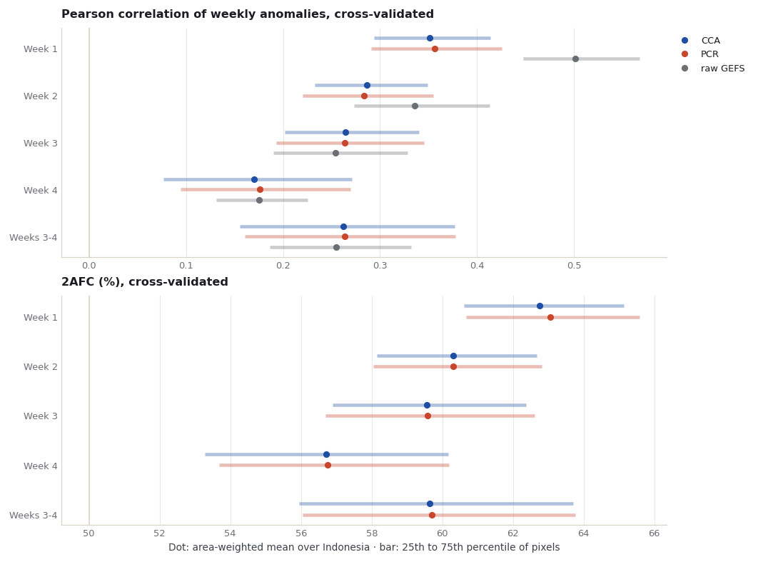
Cross-validated scores over the 249 training targets, as area-weighted means over the Indonesian pixels (weights: cosine of latitude):
Pearson correlation of hindcast and observed anomalies; 0 is no linear relationship.
2AFC: the chance (in %) that the hindcasts rank two different targets in the observed order; 50% is no skill.
ROC area for below- and above-normal weeks; 0.5 is no skill.
The raw GEFS baseline is the model’s own anomaly, interpolated linearly from 1° to the pixel centres, correlated with the observed anomalies. It involves no fitting, so it pays none of the cost that cross-validation charges the calibrated forecasts.
def clean(a):return a.where(a >-999).reindex(Y=mask["Y"], X=mask["X"], method="nearest", tolerance=1e-4).where(mask)def pearson(a, b): a, b = a - a.mean("T"), b - b.mean("T")return (a * b).sum("T") / np.sqrt((a * a).sum("T") * (b * b).sum("T"))raw_pearson = {}for lead in leads: xa = x_anom[lead].isel(T=train[7]).interp(Y=mask["Y"], X=mask["X"], method="linear") raw_pearson[lead] = pearson(xa, y_anom[days_of[lead]].isel(T=train[7])).where(mask)rows = []for (lead, method), r in results.items(): rows.append({"lead": lead, "name": lead_names[lead], "method": method,"Pearson": area(clean(r.skill_pearson)), "2AFC (%)": area(clean(r.skill_two_alternative_forced_choice)),"ROC below normal": area(clean(r.skill_roc_area_below_normal)), "ROC above normal": area(clean(r.skill_roc_area_above_normal))})for lead in leads: rows.append({"lead": lead, "name": lead_names[lead], "method": "raw GEFS", "Pearson": area(raw_pearson[lead])})order = {lead: i for i, lead inenumerate(leads)}skill_by_lead = (pd.DataFrame(rows).assign(o=lambda d: d.lead.map(order)).sort_values(["o", "method"]).drop(columns="o") .set_index(["lead", "method"]))skill_by_lead.round(3)
name
Pearson
2AFC (%)
ROC below normal
ROC above normal
lead
method
week1
CCA
Week 1
0.351
62.760
0.693
0.672
PCR
Week 1
0.356
63.056
0.696
0.678
raw GEFS
Week 1
0.501
NaN
NaN
NaN
week2
CCA
Week 2
0.287
60.317
0.658
0.639
PCR
Week 2
0.284
60.317
0.658
0.639
raw GEFS
Week 2
0.336
NaN
NaN
NaN
week3
CCA
Week 3
0.265
59.562
0.650
0.628
PCR
Week 3
0.264
59.583
0.649
0.629
raw GEFS
Week 3
0.254
NaN
NaN
NaN
week4
CCA
Week 4
0.170
56.717
0.611
0.586
PCR
Week 4
0.176
56.758
0.609
0.589
raw GEFS
Week 4
0.175
NaN
NaN
NaN
week34
CCA
Weeks 3-4
0.262
59.632
0.653
0.624
PCR
Weeks 3-4
0.264
59.692
0.653
0.628
raw GEFS
Weeks 3-4
0.255
NaN
NaN
NaN
def quartiles(field):return np.nanpercentile(field.where(mask).values, [25, 75])series = {"CCA": figures.ACCENT, "PCR": figures.MARK, "raw GEFS": figures.MUTED}panels = [("Pearson", "skill_pearson", "Pearson correlation of weekly anomalies, cross-validated", 0), ("2AFC (%)", "skill_two_alternative_forced_choice", "2AFC (%), cross-validated", 50)]fig, axes = plt.subplots(len(panels), 1, figsize=(figures.MAP_WIDTH, 7.0), layout="constrained")for ax, (column, metric, title, reference) inzip(axes, panels): ax.axvline(reference, color=figures.LINE, linewidth=1)for k, (method, colour) inenumerate(series.items()):if method =="raw GEFS"and column !="Pearson":continue offset = (k -1) *0.22for i, lead inenumerate(leads): field = raw_pearson[lead] if method =="raw GEFS"else clean(results[lead, method][metric]) low, high = quartiles(field) ax.plot([low, high], [i + offset] *2, color=colour, linewidth=3, alpha=.35, solid_capstyle="butt") ax.plot(skill_by_lead.loc[(lead, method), column], i + offset, "o", color=colour, markersize=5, label=method if i ==0elseNone) ax.set_yticks(range(len(leads)), [lead_names[lead] for lead in leads]) ax.invert_yaxis() ax.set_title(title) ax.grid(axis="y", visible=False)axes[0].legend(loc="upper left", bbox_to_anchor=(1.0, 1.0))axes[-1].set_xlabel("Dot: area-weighted mean over Indonesia · bar: 25th to 75th percentile of pixels")assets = repo /"docs/assets/week-leads-2023"assets.mkdir(parents=True, exist_ok=True)fig.savefig(assets /"skill-by-lead.png")plt.show()
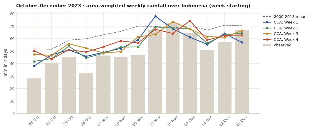
Each Wednesday from late September to late December 2023 gives a forecast for the weeks after it. A forecast total is the target’s observed 2000-2018 mean (the rule of section 4) plus the calibrated anomaly; where that sum is negative it is set to zero, and the cell counts how often.
CPT also gives tercile probabilities. It defines the categories from the training samples it was given, all 249 targets together, so the observed category uses the same definition: at each pixel, below the 33rd or above the 67th percentile of the 249 training anomalies (NumPy’s hazen rule, as in chapter 5).
test_T = all_T[~train[7]]observed, observed_anom, clim_2023, category = {}, {}, {}, {}for days in (7, 14): observed[days] = obs[days].isel(T=~train[days]).where(mask) clim_2023[days] = y_clim[days].isel(T=~train[days]) observed_anom[days] = y_anom[days].isel(T=~train[days]) lo, hi = np.quantile(y_anom[days].isel(T=train[days]).values, [0.33, 0.67], axis=0, method="hazen") lower = xr.DataArray(lo, coords={"Y": mask["Y"], "X": mask["X"]}, dims=("Y", "X")) upper = lower.copy(data=hi) a = observed_anom[days] category[days] = xr.where(a < lower, 0, xr.where(a > upper, 2, 1)).where(a.notnull())forecast, clipped = {}, {}for (lead, method), r in results.items(): days = days_of[lead] anomaly = clean(r.deterministic).assign_coords(T=test_T) total = clim_2023[days] + anomaly clipped[lead, method] =int((total <0).sum()) probability = clean(r.probabilistic).assign_coords(T=test_T) most_likely = probability.fillna(-1).argmax("C").where(probability.notnull().all("C") & mask) forecast[lead, method] =dict(total=total.clip(min=0).where(mask), probability=probability, most_likely=most_likely, top=probability.max("C").where(mask))print("Forecast totals below zero before clipping (pixel-targets):", {f"{lead}-{m}": n for (lead, m), n in clipped.items()},f"of {int(mask.sum()) *len(test_T):,} per lead")issues = {}for r in design[design.kind =="forecast"].sort_values(["start", "first_day"]).itertuples(): issues.setdefault(r.start, []).append((r.lead, r.target))print(f"{len(issues)} Wednesdays in 2023 with at least one target; complete issues (all five leads): "f"{sum(len(v) ==len(leads) for v in issues.values())}")for s, items inlist(issues.items())[:3]:print(f" issued {s:%a %d %b}: "+", ".join(f"{lead_names[lead]} from {t:%d %b}"for lead, t in items))
Forecast totals below zero before clipping (pixel-targets): {'week1-CCA': 4627, 'week1-PCR': 9415, 'week2-CCA': 3669, 'week2-PCR': 9615, 'week3-CCA': 3024, 'week3-PCR': 4970, 'week4-CCA': 3597, 'week4-PCR': 4534, 'week34-CCA': 2418, 'week34-PCR': 3662} of 795,470 per lead
16 Wednesdays in 2023 with at least one target; complete issues (all five leads): 10
  issued Wed 13 Sep: Week 4 from 05 Oct
  issued Wed 20 Sep: Week 3 from 05 Oct, Weeks 3-4 from 05 Oct, Week 4 from 12 Oct
  issued Wed 27 Sep: Week 2 from 05 Oct, Week 3 from 12 Oct, Weeks 3-4 from 12 Oct, Week 4 from 19 Oct
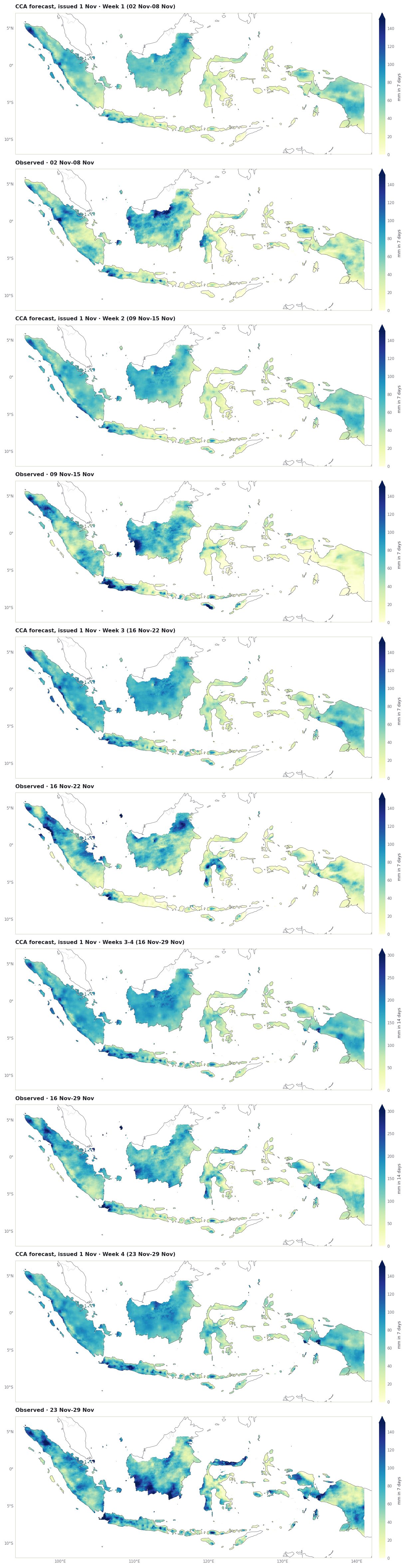
One issue date in full: the forecast issued on Wednesday 1 November 2023 (the issue date of the monthly and seasonal cases) for each lead, with the observation below each forecast. One column.
example = pd.Timestamp("2023-11-01")fig, grid = figures.stacked([figures.map_height(predictand_box)] * (2*len(leads)))row =0for lead, target in issues[example]: days = days_of[lead] end = target + pd.Timedelta(days=days -1) vmax =150if days ==7else300for label, field in [(f"CCA forecast, issued 1 Nov · {lead_names[lead]} ({target:%d %b}-{end:%d %b})", forecast[lead, "CCA"]["total"].sel(T=target)), (f"Observed · {target:%d %b}-{end:%d %b}", observed[days].sel(T=target))]: ax = figures.map_axes(fig, grid[row, 0], predictand_box, bottom_labels=row ==2*len(leads) -1) image = figures.draw_field(ax, field, cmap="YlGnBu", vmin=0, vmax=vmax) ax.set_title(label) figures.colorbar(fig, image, ax, f"mm in {days} days", extend="max") row +=1fig.savefig(assets /"issued-2023-11-01.png")plt.show()
The same issue date in numbers: for each lead, the forecast and observed totals averaged over Indonesia (area-weighted), the 2000-2018 mean, and how well the most likely category matched what happened. One issue date is one outcome per lead, not a skill estimate.
rows = []for item in issues[example]: lead, target = item[0], item[1] days = days_of[lead] end = target + pd.Timedelta(days=days -1) obs_t, clim_t, cat_t = observed[days].sel(T=target), clim_2023[days].sel(T=target), category[days].sel(T=target) w = (weights * cat_t.notnull()).astype(float) shares = {name: float(w.where(cat_t == k, 0).sum() / w.sum() *100) for k, name inenumerate(["below", "near", "above"])}for m in ["CCA", "PCR"]: f = forecast[lead, m] ml = f["most_likely"].sel(T=target) wm = w.where(ml.notnull(), 0) rows.append({"lead": lead, "name": lead_names[lead], "method": m, "target": f"{target:%d %b}-{end:%d %b %Y}","forecast mean (mm)": float(f["total"].sel(T=target).weighted(wm).mean()),"observed mean (mm)": float(obs_t.weighted(wm).mean()),"2000-2018 mean (mm)": float(clim_t.where(mask).weighted(wm).mean()),"hit rate (%)": float(wm.where(ml == cat_t, 0).sum() / wm.sum() *100),"reference hit rate (%)": max(shares.values()),**{f"observed {k} (%)": v for k, v in shares.items()},**{f"forecast {name} (%)": float(wm.where(ml == k, 0).sum() / wm.sum() *100)for k, name inenumerate(["below", "near", "above"])}})headline = pd.DataFrame(rows).set_index(["lead", "method"])headline.round(1)
name
target
forecast mean (mm)
observed mean (mm)
2000-2018 mean (mm)
hit rate (%)
reference hit rate (%)
observed below (%)
observed near (%)
observed above (%)
forecast below (%)
forecast near (%)
forecast above (%)
lead
method
week1
CCA
Week 1
02 Nov-08 Nov 2023
48.9
46.2
63.0
51.0
52.4
52.4
40.0
7.6
95.7
3.3
1.0
PCR
Week 1
02 Nov-08 Nov 2023
48.6
46.2
63.0
51.2
52.4
52.4
40.0
7.6
93.5
4.9
1.6
week2
CCA
Week 2
09 Nov-15 Nov 2023
53.1
44.9
65.7
57.8
58.6
58.6
31.7
9.7
95.2
3.6
1.2
PCR
Week 2
09 Nov-15 Nov 2023
52.7
44.9
65.7
54.8
58.6
58.6
31.7
9.7
92.6
4.8
2.6
week3
CCA
Week 3
16 Nov-22 Nov 2023
61.3
47.0
69.8
63.8
68.3
68.3
20.5
11.2
83.8
10.8
5.4
PCR
Week 3
16 Nov-22 Nov 2023
61.0
47.0
69.8
61.8
68.3
68.3
20.5
11.2
81.3
11.4
7.3
week34
CCA
Weeks 3-4
16 Nov-29 Nov 2023
131.2
113.8
139.6
47.6
54.5
54.5
31.8
13.7
65.0
26.7
8.3
PCR
Weeks 3-4
16 Nov-29 Nov 2023
131.2
113.8
139.6
45.0
54.5
54.5
31.8
13.7
62.8
23.2
14.0
week4
CCA
Week 4
23 Nov-29 Nov 2023
67.4
66.8
69.7
34.0
36.4
35.2
36.4
28.3
13.6
31.5
54.9
PCR
Week 4
23 Nov-29 Nov 2023
67.4
66.8
69.7
33.1
36.4
35.2
36.4
28.3
28.8
20.1
51.1
Over all 13 targets of 2023, for each lead: the area-weighted forecast total against the observed total, then scores over every pixel and target (area-weighted):
Hit rate: share where the most likely category was the one observed. The reference is the share of the most frequent observed category.
RPSS 2023: ranked probability skill score against climatological odds (33/34/33%); above 0 is closer to what happened. Thirteen weeks of one season, not a skill estimate.
RMSE 2023: error of the forecast totals in mm.
def rps(probability, cat): cumulative = probability.cumsum("C") /100 outcome = xr.concat([(cat <= k).astype(float) for k inrange(3)], dim="C").assign_coords(C=probability["C"])return ((cumulative - outcome) **2).isel(C=slice(0, 2)).sum("C")rows, references = [], {}for days in (7, 14): w3 = (weights * category[days].notnull()).astype(float) references[days] = {name: float(w3.where(category[days] == k, 0).sum() / w3.sum() *100)for k, name inenumerate(["below normal", "near normal", "above normal"])}for (lead, method), f in forecast.items(): days = days_of[lead] w = (weights * category[days].notnull()).where(f["most_likely"].notnull(), 0).astype(float) climatology = xr.DataArray([33.0, 34.0, 33.0], dims="C", coords={"C": f["probability"]["C"]}).broadcast_like(f["probability"]) rows.append({"lead": lead, "name": lead_names[lead], "method": method,"hit rate (%)": float(w.where(f["most_likely"] == category[days], 0).sum() / w.sum() *100),"reference hit rate (%)": max(references[days].values()),"RPSS 2023": float(1- rps(f["probability"], category[days]).weighted(w).mean()/ rps(climatology, category[days]).weighted(w).mean()),"RMSE 2023 (mm)": float(np.sqrt(((f["total"] - observed[days]) **2).weighted(w).mean())),"mean forecast (mm)": float(f["total"].weighted(w).mean()),"observed mean (mm)": float(observed[days].weighted(w).mean()),**{f"forecast {name} (%)": float(w.where(f["most_likely"] == k, 0).sum() / w.sum() *100)for k, name inenumerate(["below", "near", "above"])}})forecast_2023 = (pd.DataFrame(rows).assign(o=lambda d: d.lead.map(order)).sort_values(["o", "method"]).drop(columns="o") .set_index(["lead", "method"]))print("Observed categories, share of area x targets (%):", {d: {k: round(v, 1) for k, v in r.items()} for d, r in references.items()})forecast_2023.round(2)
Observed categories, share of area x targets (%): {7: {'below normal': 49.3, 'near normal': 32.5, 'above normal': 18.1}, 14: {'below normal': 52.2, 'near normal': 30.7, 'above normal': 17.1}}
Tables and figures for the story page, a NetCDF file of the skill maps, and the fields of the interactive page. At 0.05° every map has about 61,000 values, so the page reads small binary files, one per map, only when a view needs them: integers at a stated scale, stored only at the Indonesian pixels in the order of a shared pixel list, and gzip-compressed.
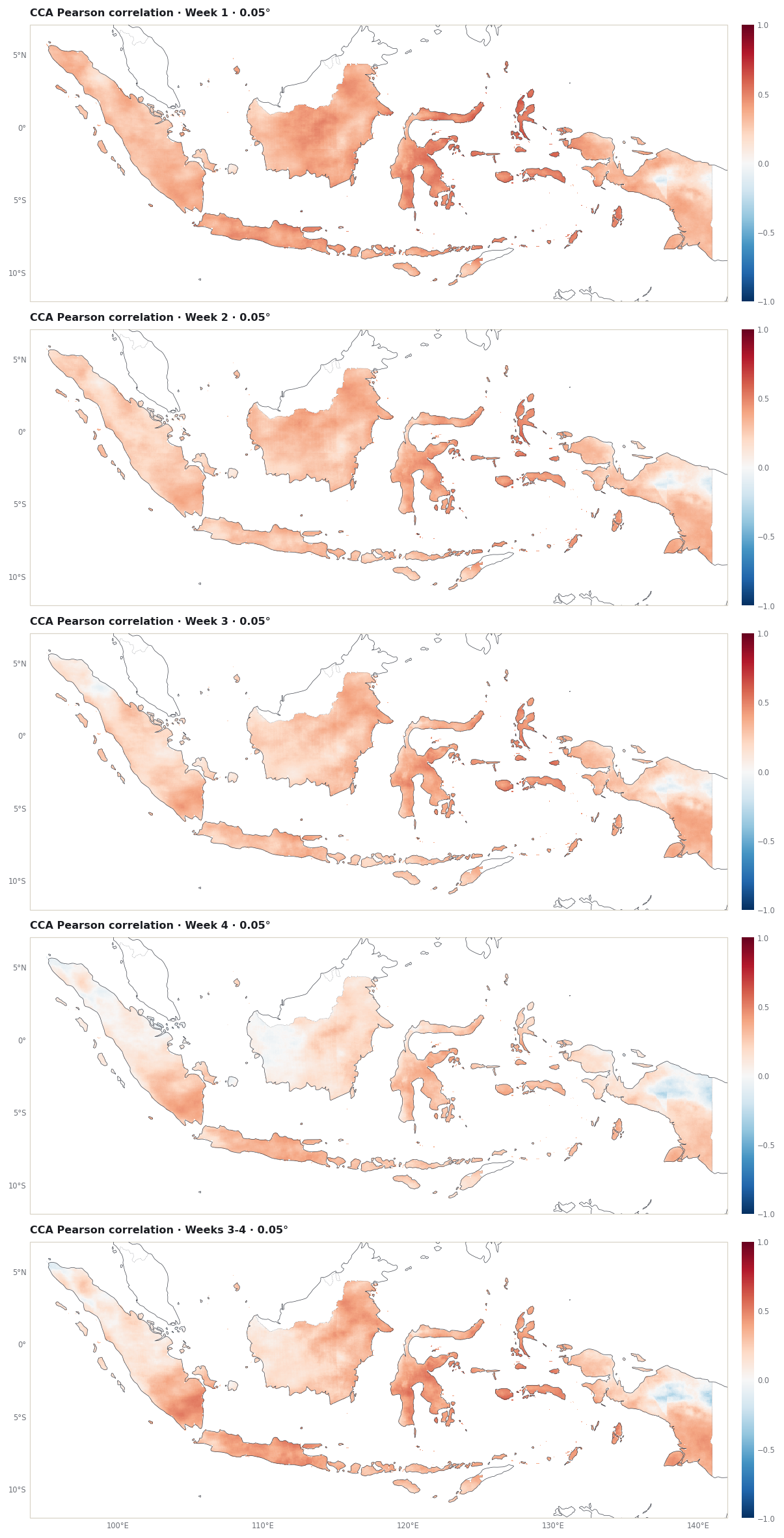
data_dir = repo /"docs/data/week-leads-2023"data_dir.mkdir(parents=True, exist_ok=True)skill_by_lead.round(4).to_csv(data_dir /"skill-by-lead.csv")headline.round(4).to_csv(data_dir /f"issued-{example:%Y-%m-%d}.csv")forecast_2023.round(4).to_csv(data_dir /"ond-2023-weekly-forecasts.csv")design.assign(**{c: design[c].dt.date for c in ["target", "end", "start"]}).to_csv(data_dir /"lead-design.csv", index=False)area_rows = {"week starting": [str(pd.Timestamp(t).date()) for t in test_T], "observed": observed_series.values, "mean_2000_2018": clim_series.values}for lead in week_leads: area_rows[f"cca_total_{lead}"] = forecast[lead, "CCA"]["total"].weighted(weights).mean(("Y", "X")).valuespd.DataFrame(area_rows).round(3).to_csv(data_dir /"ond-2023-area-totals.csv", index=False)summary = {"target": "October-December 2023, weekly", "model": "GEFSv12 (IRI SubX GEFSv12_CPC)", "grid": "CHIRPS v3.0 native 0.05 degree","issue_rule": "issued Wednesday 00 UTC; week 1-4 = days 1-7, 8-14, 15-21, 22-28; weeks 3-4 = days 15-28","training_years": [training_years[0], training_years[-1]], "training_targets_per_lead": int(train[7].sum()),"pixels": int(mask.sum()), "cross_validation_window": settings["crossvalidation_window"],"settings": {k: str(v) for k, v in cca_settings.items()},"observed_category_percent_2023": {f"{d}-day": {k: round(v, 2) for k, v in r.items()} for d, r in references.items()},"fit_minutes": {f"{lead}-{m}": round(r.attrs["fit_seconds"] /60, 1) for (lead, m), r in results.items()},"clipped_pixel_targets": {f"{lead}-{m}": n for (lead, m), n in clipped.items()}}(data_dir /"summary.json").write_text(json.dumps(summary, indent=2) +"\n")maps = xr.Dataset()for lead in leads:for m in ["CCA", "PCR"]: maps[f"{m.lower()}_pearson_{lead}"] = clean(results[lead, m].skill_pearson).drop_vars( [c for c in results[lead, m].skill_pearson.coords if c notin ("Y", "X")], errors="ignore").astype("float32") maps[f"raw_pearson_{lead}"] = raw_pearson[lead].astype("float32")_ = save_netcdf(maps, data_dir /"week-leads-2023-skill-maps.nc", overwrite=True, metadata={"note": "Weekly rainfall, GEFSv12 week 1-4 and weeks 3-4: cross-validated correlation 2000-2018 at 0.05 degree"})
# Interactive fields: one gzip-compressed binary file per mapfield_dir = assets /"fields"field_dir.mkdir(exist_ok=True)for old in field_dir.glob("*"): old.unlink()north = mask.transpose("Y", "X").valuesflat = np.flatnonzero(north.ravel()) # row 0 = northernmost pixel rown =len(flat)def at_pixels(a):return np.asarray(a.transpose("Y", "X").values, dtype="float64").ravel()[flat]def encode(values, kind, scale): v = np.round(values * scale)if kind =="i16":return np.where(np.isfinite(v), np.clip(v, -32767, 32767), -32768).astype("<i2").tobytes()if kind =="u16":return np.where(np.isfinite(v), np.clip(v, 0, 65534), 65535).astype("<u2").tobytes()return np.where(np.isfinite(v), np.clip(v, 0, 254), 255).astype("u1").tobytes()def write(name, parts): blob =b"".join(encode(*p) for p in parts) (field_dir /f"{name}.bin.gz").write_bytes(gzip.compress(blob, 9, mtime=0))(assets /"pixels.bin").write_bytes(flat.astype("<i4").tobytes())for lead in leads:for m in ["CCA", "PCR"]: write(f"skill-{m}-pearson-{lead}", [(at_pixels(clean(results[lead, m].skill_pearson)), "i16", 1000)]) write(f"skill-{m}-twoafc-{lead}", [(at_pixels(clean(results[lead, m].skill_two_alternative_forced_choice)), "i16", 10)]) write(f"skill-raw-pearson-{lead}", [(at_pixels(raw_pearson[lead]), "i16", 1000)])for days in (7, 14):for t in test_T: key =f"{pd.Timestamp(t):%Y-%m-%d}" write(f"obs-{days}-{key}", [(at_pixels(observed[days].sel(T=t)), "u16", 10), (at_pixels(clim_2023[days].sel(T=t).where(mask)), "u16", 10), (at_pixels(category[days].sel(T=t)), "u8", 1)])for (lead, m), f in forecast.items():for t in test_T: key =f"{pd.Timestamp(t):%Y-%m-%d}" write(f"fc-{lead}-{m}-{key}", [(at_pixels(f["total"].sel(T=t)), "u16", 10), (at_pixels(f["most_likely"].sel(T=t)), "u8", 1), (at_pixels(f["top"].sel(T=t)), "u8", 1)])def records(frame):return [{k: (Noneifisinstance(v, float) andnot np.isfinite(v) else v) for k, v in row.items()}for row in frame.to_dict(orient="records")]manifest = {"grid": {"west": round(float(mask.X.min()) -.025, 3), "north": round(float(mask.Y.max()) +.025, 3), "step": 0.05,"nx": int(mask.sizes["X"]), "ny": int(mask.sizes["Y"]), "pixels": n},"leads": list(range(1, len(leads) +1)), "leadKeys": leads, "leadNames": [lead_names[lead] for lead in leads],"days": {lead: days_of[lead] for lead in leads},"firstDay": {lead: weeks.LEADS[lead][0] for lead in leads},"methods": ["CCA", "PCR"], "rawName": "raw GEFS", "training": "2000-2018","sample": "the 249 training targets of 2000-2018", "cellText": f"Indonesia's {n:,} pixels at 0.05°","layout": {"skill": [["value", "i16"]], "obs": [["total", "u16", 10], ["mean", "u16", 10], ["category", "u8", 1]],"fc": [["total", "u16", 10], ["category", "u8", 1], ["probability", "u8", 1]]},"scales": {"pearson": 1000, "twoafc": 10},"issues": [{"issued": f"{s:%Y-%m-%d}", "label": f"{s:%a %d %b %Y}","targets": [{"lead": lead, "start": f"{t:%Y-%m-%d}", "days": days_of[lead]} for lead, t in items]}for s, items in issues.items()],"skillTable": records(skill_by_lead.reset_index().rename(columns={"lead": "leadKey"}).assign( lead=lambda d: d.leadKey.map(order) +1).round(4)),"scores2023": records(forecast_2023.reset_index().round(3)),"headline": {"issued": f"{example:%Y-%m-%d}", "rows": records(headline.reset_index().round(3))},"series": pd.DataFrame(area_rows).round(2).to_dict(orient="list"),"rainMax": {days: float(np.ceil(np.nanpercentile(np.concatenate( [observed[days].values.ravel()] + [forecast[lead, m]["total"].values.ravel() for lead in leads for m in ["CCA", "PCR"] if days_of[lead] == days]),99) /50) *50) for days in (7, 14)},}(assets /"manifest.json").write_text(json.dumps(manifest, separators=(",", ":"), allow_nan=False) +"\n")sizes =sorted(p.stat().st_size for p in field_dir.iterdir())print(f"{n:,} pixels; {len(sizes)} field files, {sum(sizes) /1e6:.1f} MB in total (largest {sizes[-1] /1e3:.0f} kB); "f"manifest {(assets /'manifest.json').stat().st_size /1e3:.0f} kB")for f insorted(data_dir.iterdir()) +sorted(p for p in assets.iterdir() if p.is_file()):print(f"{f.relative_to(repo)} ({f.stat().st_size /1000:.0f} kB)")
IRI Data Library. SubX EMC GEFSv12_CPC (hindcast and forecast precipitation). https://iridl.ldeo.columbia.edu/SOURCES/.Models/.SubX/.EMC/.GEFSv12_CPC/ Browsing Data Library pages requires signing in (checked 10 November 2026); PyCPT’s data requests in this tutorial succeeded without a key.
Guan, H., Zhu, Y., Sinsky, E., et al. (2022). GEFSv12 reforecast dataset for supporting subseasonal and hydrometeorological applications. Monthly Weather Review, 150(3), 647-665. https://doi.org/10.1175/MWR-D-21-0245.1
NOAA Climate Prediction Center. Week 3-4 Outlooks (issued on Fridays; the outlook shown on 11 November 2026 was issued Friday 6 November 2026 for 21 November to 4 December, days 15 to 28 after issue). https://www.cpc.ncep.noaa.gov/products/predictions/WK34/
Climate Hazards Center, UC Santa Barbara. CHIRPS: Rainfall Estimates from Rain Gauge and Satellite Observations (CHIRPS version 3.0 page). https://www.chc.ucsb.edu/data/chirps3
Funk, C., Peterson, P., Landsfeld, M., et al. (2014). A quasi-global precipitation time series for drought monitoring. U.S. Geological Survey Data Series 832. https://doi.org/10.3133/ds832
Mason, S. J., and Weigel, A. P. (2009). A generic forecast verification framework for administrative purposes. Monthly Weather Review, 137(1), 331-349. https://doi.org/10.1175/2008MWR2553.1