CCA, PCR, raw CFSv2 and climatology · seasons centred on 2023
This companion notebook teaches the analysis of forecasts produced through PyCPT. Reading its already-executed outputs requires only a browser. Running the default cells uses saved results and scientific Python packages: no PyCPT installation, CPT executable, IRI Data Library credentials, data downloads or new fitting are required. Use the complete tutorial kit, which includes the data and helper code.
An optional OND section shows the actual PyCPT calibration calls. That extension requires PyCPT with its compatible CPT engine; it uses local inputs and needs no IRI Data Library authentication. Outputs go to temp/, preserving the research archive.
Learning goals. Select target seasons without a year-label error; compare four forecast methods on identical country-land cells; calculate spatial errors; inspect geographic differences; distinguish training sensitivity from independent evidence.
1. Find the project and check the teaching data
Run from the repository or tutorial-kit folder, or a directory beneath it. The notebook discovers that root so it also works when Jupyter starts in docs/notebooks/. For default execution, select a kernel with NumPy, pandas, xarray, Matplotlib, netCDF4 and IPython installed. The kit’s environment/offline-analysis.yml provides the scientific-Python package specification; Python (Tutorial Analysis) is the suggested kernel name. An existing working tutorial kernel can also be used. PyCPT and its CPT executable are needed only if you enable the optional refit. Hash verification detects changed data before calculating results.
from pathlib import Pathimport sysroot =next((p for p in (Path.cwd(), *Path.cwd().parents)if (p /"pycpt_tutorial").is_dir() and (p /"docs/data").is_dir()), None)if root isNone:raiseFileNotFoundError("Open this notebook inside the full repository or extracted tutorial kit.")sys.path.insert(0, str(root))import jsonimport hashlibimport datetime as dtimport numpy as npimport pandas as pdimport xarray as xrimport matplotlib.pyplot as pltfrom IPython.display import display, HTMLfrom pycpt_tutorial import teaching as teachfrom pycpt_tutorial.export import save_netcdf%matplotlib inlineteach.style()data_dir = root /"docs/data"artifacts = root /"docs/assets/seasonal-2023"artifacts.mkdir(parents=True, exist_ok=True)provenance = teach.verify_bundle(data_dir)def load(name):with xr.open_dataset(data_dir / name) as source:return source.load()data = load("indonesia-seasons-2023.nc")context = load("verification-context-2021-2024.nc")print(f"Verified {len(provenance['outputs'])} input files; {int(data.evaluation_mask.sum()):,} country-land cells.")
Verified 5 input files; 3,240 country-land cells.
2. Keep actual dates visible
A season is a three-month rainfall total, not a single month. This tutorial orders seasons by their midpoint in 2023. DJF spans December 2022–February 2023; NDJ spans November 2023–January 2024. The research archive uses ending-year labels, so that last window is stored as NDJ 2024. Keep this source label unchanged.
Each forecast was initialized on the first day of the month before its target begins. The three CFSv2 lead centres are 1.5, 2.5 and 3.5 months. Monthly rates were integrated with actual month lengths before this teaching copy was made.
Observation: local CHIRPS3 rainfall, aggregated from 0.05° to 0.25° country-land means. It is a gridded observational estimate, not independent station validation. Raw: the same CFSv2 ensemble-mean seasonal forecast supplied at 1°, interpolated to the observation grid. A 0.25° output does not establish 0.25° dynamical skill.
Climatology: the mean observed total over the fitting period, unchanged from year to year. CCA/PCR: regression-calibrated forecasts, each trained separately for each target season. The main illustration uses 1991–2020; 1983–2010 is a sensitivity check. This choice is stated upfront rather than selecting a different winner each season.
The fits retain three predictor EOFs; CCA additionally retains three predictand EOFs and two CCA modes. Counts are fixed, not optimized. CPT used synchronous predictors and five-sample cyclic CV, refitting within folds, then fitted the full training period for the later forecasts. No transform, tailoring, dry mask or skill mask was enabled. CPT automatically zero-bounds rainfall. These are current-vintage retrospective replays.
mask = data.evaluation_mask.astype(bool)weights = data.evaluation_weight.where(mask, 0)weights = weights / weights.sum(("Y", "X"))assertint(mask.sum()) ==3240assert np.isclose(float(weights.sum()), 1)assertint(data.forecast_rainfall.count()) ==12*7*3240assertint(data.observed_rainfall.count()) ==12*3240main_variants = teach.MAINprint("Same observations, 3,240 cells and normalized country-land weights for every method.")
Same observations, 3,240 cells and normalized country-land weights for every method.
4. Calculate errors, rather than ranking maps by appearance
For each seasonal window and forecast, calculate \(e_i=f_i-o_i\), \(\mathrm{RMSE}=\sqrt{\sum_i w_i e_i^2}\), \(\mathrm{MAE}=\sum_i w_i|e_i|\), and \(\mathrm{bias}=\sum_i w_i e_i\). The weights sum to one. Positive bias means a forecast is too wet.
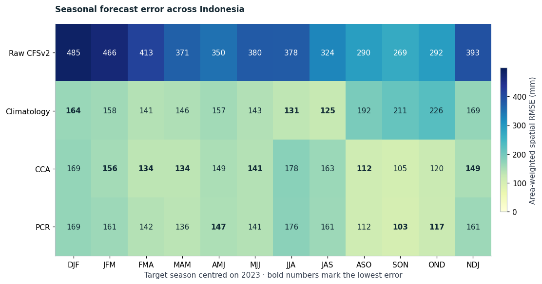
These are spatial scores across Indonesia for one seasonal forecast, not the error of a national-mean time series. RMSE penalizes large local errors strongly. Assertions below independently reproduce the saved scores for every selected window, including NDJ’s different source year.
Figure 17.1: Spatial RMSE across the twelve seasons centred on 2023. Lower is better; bold entries identify the lowest unrounded score in each season. All methods use the same country-land cells and weights.
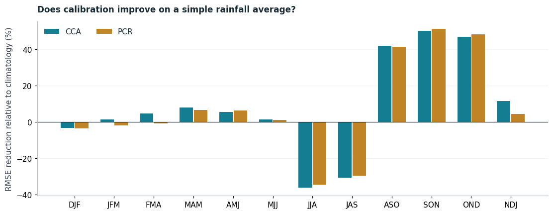
A calibrated forecast should be compared with both the raw model and climatology. Correcting a large raw bias does not automatically beat a simple observed average. The following reduction is \(100(1-\mathrm{RMSE}_{model}/\mathrm{RMSE}_{climo})\). It is an RMSE reduction, not a ranked probability skill score or a significance test.
Figure 17.2: RMSE reduction relative to the 1991–2020 climatology forecast. Positive values mean lower error after calibration; negative values favour climatology.
5. Walk through OND before looking across every season
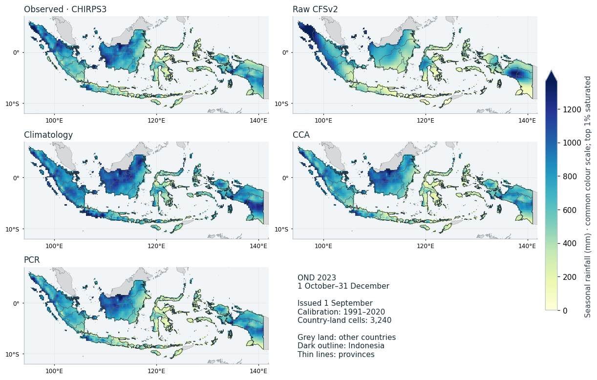
OND 2023 was initialized on 1 September and verifies over 1 October–31 December. Read the five maps on the same rainfall scale. CHIRPS3 is the verification reference; the other panels are forecasts. More spatial detail is not itself evidence of better forecasts. The common scale saturates its highest 1% to keep lower totals legible.
Figure 17.3: OND 2023 observed and forecast rainfall on a common scale. Only country-land cells are shaded. The upper 1% is saturated for display; numeric files retain all values. Grey land shows other countries; Indonesia has no boundary fill, with dark country and thin province outlines.
Inspect the actual fitting inputs
These NetCDF files are lossless teaching copies of the native CPT text inputs. They retain the forecast initialization and target coordinates and the missing-value metadata required by cptcore. Predictors and observations have different spatial grids; their training target dates must match. The observation mean also checks the OND climatology baseline (within the native text’s printed precision).
X: {'T': 30, 'Y': 41, 'X': 71}; Y: {'T': 30, 'Y': 76, 'X': 192}; F: {'T': 1, 'Y': 41, 'X': 71}
Training and forecast dates are separate; climatology check passed.
Optional: rerun CCA and PCR in new scratch directories
Keep RERUN_CPT = False for the default offline analysis, which needs no PyCPT or CPT installation. Set it to True only in the tested PyCPT fitting environment, after conda activation sets CPT_BIN_DIR for the compatible engine. The supplied fitting setup is PyCPT 2.10.4, cptio 1.4.0 and CPT 17.8.3. All OND inputs are local; no IRI Data Library authentication is needed for this refit.
The visible settings below reproduce the fixed-mode design. The scoped reader handles the audited initialization-date headers without changing forecast numbers. This refits OND only, not all twelve seasons. New logs and outputs go to a unique temp/ directory. Returned forecasts are checked against the saved case before export. The first published execution uses saved results; the optional path is tested separately.
RERUN_CPT =Falseif RERUN_CPT:from cptcore import canonical_correlation_analysis, principal_components_regressionfrom pycpt_tutorial.cpt_dates import verified_midnight_readerimport tempfile (root /"temp").mkdir(exist_ok=True) work = Path(tempfile.mkdtemp(prefix="ond-tutorial-", dir=root /"temp")) settings =dict(x_eof_modes=(3, 3), validation="CROSSVALIDATION", crossvalidation_window=5, synchronous_predictors=True, transform_predictand=None, tailoring=None, drymask_threshold=None, skillmask_threshold=None) expected_dates = [pd.Timestamp(v).to_pydatetime() for v in np.concatenate([X.S.values, F.S.values])]for method, function in (("cca", canonical_correlation_analysis), ("pcr", principal_components_regression)): options =dict(settings)if method =="cca": options.update(y_eof_modes=(3, 3), cca_modes=(2, 2))with verified_midnight_reader(function, expected_dates): result = function(X, Y, F=F, **options, cpt_kwargs={"outputdir": work / method, "log": work /f"{method}.log","project_file": work /f"{method}-commands.txt"}) forecast = result[1].reindex(X=data.X, Y=data.Y, method="nearest", tolerance=1e-3).where(mask) saved = data.forecast_rainfall.sel(season="OND", forecast_variant=f"{method}_1991_2020") np.testing.assert_allclose(forecast.deterministic.isel(T=0), saved, atol=.01, rtol=0, equal_nan=True) save_netcdf(forecast, work /f"{method}-forecast.nc", overwrite=False)print(f"CCA/PCR reruns match saved OND forecasts; new outputs: {work}")else:print("Calibration rerun skipped; all comparisons use the hash-verified saved results.")
Calibration rerun skipped; all comparisons use the hash-verified saved results.
6. Inspect geographic differences across all twelve seasons
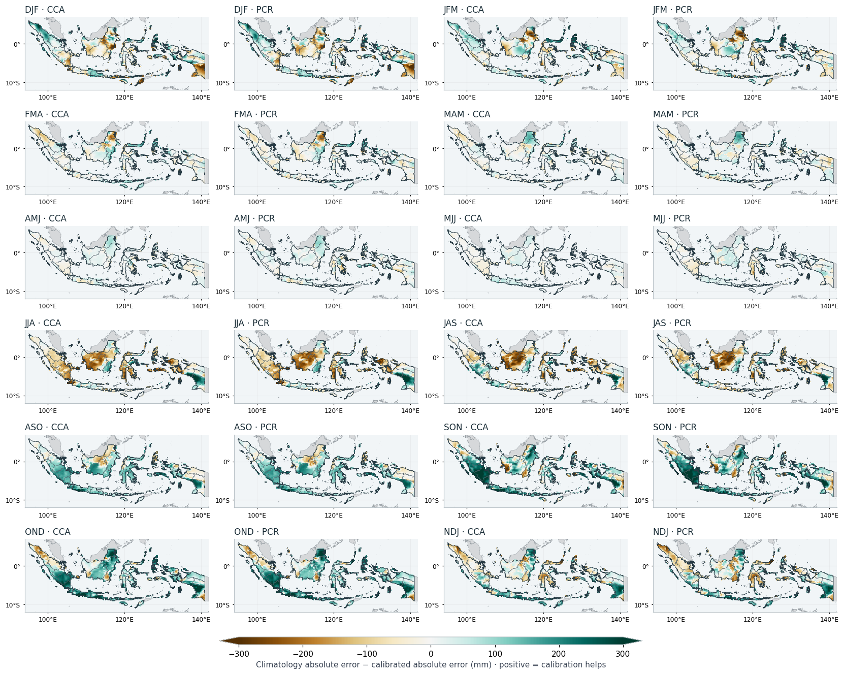
Subtract each calibrated absolute error from climatology’s absolute error at the same cell. Positive values mean calibration helped there; negative values mean climatology did better. A lower national RMSE can coexist with local deterioration. The atlas shows both models for every season, rather than selecting only favourable maps. Colours saturate beyond ±300 mm; downloadable numeric fields retain all values.
reference_error =abs(error.sel(forecast_variant="climatology_1991_2020"))local_gain = reference_error -abs(error.sel(forecast_variant=["cca_1991_2020", "pcr_1991_2020"]))local_gain.attrs.update(units="mm", long_name="Absolute-error reduction relative to climatology")save_netcdf(local_gain.rename("absolute_error_reduction"), artifacts /"local-error-reduction-2023.nc", metadata={"units": "mm", "positive_means": "Calibration has smaller absolute error than climatology"}, overwrite=True)fig = teach.error_atlas(data)teach.save_figure(fig, artifacts, "error-atlas")plt.show()
Figure 17.4: Local absolute-error reduction relative to climatology for CCA and PCR in every season. Green means calibration helps, brown means it worsens the local forecast; colours saturate beyond ±300 mm. Grey land shows other countries; Indonesia has no boundary fill, with dark country and thin province outlines.
7. Compare provinces on the existing forecast grid
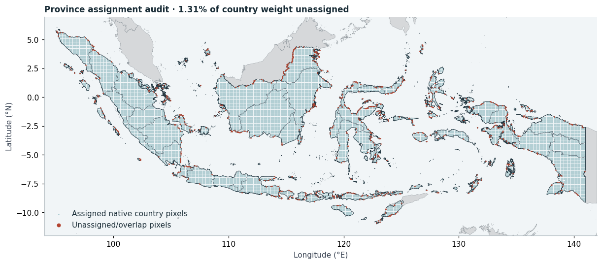
The supplied file contains 38 provinces. We define the regions from these boundaries before inspecting their forecast errors, and keep every province. Analysis uses the unsimplified polygons, not the display GeoJSON. A native 0.05° pixel is assigned only when its centre lies inside exactly one province; gaps or overlaps remain separate categories. Cosine-latitude weights are the same as in the original country aggregation. See the weighting example and point-containment definition.
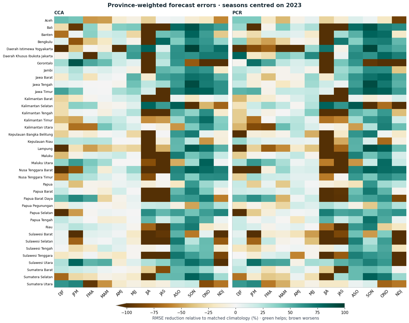
These are province-weighted scores of the saved 0.25° cell errors. Where a coarse cell crosses a province border, provinces share that cell’s forecast and observation error, but receive different native-pixel weight shares. This does not reconstruct province-only rainfall inside that cell or create finer forecast information. Small provinces need particular care. The boundary snapshot is not a certification of current or historical official administrative limits.
region_dir = data_dir /'regions'region_provenance = json.loads((region_dir /'provenance.json').read_text())for name, record in region_provenance['outputs'].items():assert hashlib.sha256((region_dir / name).read_bytes()).hexdigest() == record['sha256'], namedef load_region(name):with xr.open_dataset(region_dir / name) as source:return source.load()regions = load_region('province-weights.nc')native_membership = load_region('native-membership.nc')regional_annual = load_region('province-context-annual.nc')regional_pooled = load_region('province-context-pooled.nc')province_names = regions.region.values[regions.is_province.values.astype(bool)].tolist()assertlen(province_names) ==38np.testing.assert_allclose(regions.region_weight.sum('region'), data.evaluation_weight, atol=1e-12, rtol=0)region_mass = regions.region_weight.sum(('Y','X'))region_fraction = region_mass / region_mass.sum()unassigned_fraction = region_provenance['unassigned_weight_fraction']print(f"All 38 provinces retained; {100*unassigned_fraction:.2f}% of country weight unassigned; "f"{region_provenance['overlap_points']} overlapping native points. No nearest-province assignment.")
All 38 provinces retained; 1.31% of country weight unassigned; 0 overlapping native points. No nearest-province assignment.
Figure 17.5: Native country-pixel assignment to the supplied provinces. Red points remain an explicit residual category; the original national footprint is preserved.
Normalize the weight within each region, then calculate the same spatial MSE, RMSE, MAE and bias as before. For regional weight fraction \(a_r\), national MSE must equal \(\sum_r a_r\,\mathrm{MSE}_r\), including the residual category. National RMSE is the square root of that result, not an average of province RMSEs. The following code checks the identity and the archived regional scores.
regional_weights = regions.region_weight / region_massregional = xr.Dataset({'mse': (error.fillna(0)**2* regional_weights).sum(('Y','X')),'mae': (abs(error.fillna(0)) * regional_weights).sum(('Y','X')),'bias': (error.fillna(0) * regional_weights).sum(('Y','X')),})regional['rmse'] = np.sqrt(regional.mse)for variable in regional: regional[variable].attrs['units'] ='mm2'if variable =='mse'else'mm'for variable in ('rmse','mae','bias'): combined = np.sqrt((regional.mse*region_fraction).sum('region')) if variable=='rmse'else (regional[variable]*region_fraction).sum('region') np.testing.assert_allclose(combined, scores[variable], atol=1e-8, rtol=0)for season in teach.SEASONS: selected = regional_annual.sel(season=season, season_year=int(data.source_season_year.sel(season=season)))for variable in regional: xr.testing.assert_allclose(regional[variable].sel(season=season, drop=True).reset_coords(drop=True), selected[variable].reset_coords(drop=True))save_netcdf(regional, artifacts /'province-verification-2023.nc', overwrite=True, metadata={'scope':'Province-weighted views of existing 0.25degree errors; includes unassigned residual','calendar':'Target midpoints2023, NDJ source ending-year2024'})regional.to_dataframe().reset_index().to_csv(artifacts /'province-metrics-2023.csv', index=False)regional_annual.to_dataframe().reset_index().to_csv(artifacts /'province-metrics-context-annual.csv', index=False)regional_pooled.to_dataframe().reset_index().to_csv(artifacts /'province-metrics-context-pooled.csv', index=False)print('Province plus residual MSE, MAE and bias reproduce the national scores.')
Province plus residual MSE, MAE and bias reproduce the national scores.
Figure 17.6: RMSE reductions for CCA and PCR relative to 1991–2020 climatology in every supplied province. Green means smaller error, brown larger error. Values below −100% saturate; files retain all values. These are weights on existing 0.25° errors, not finer province rainfall reconstructions.
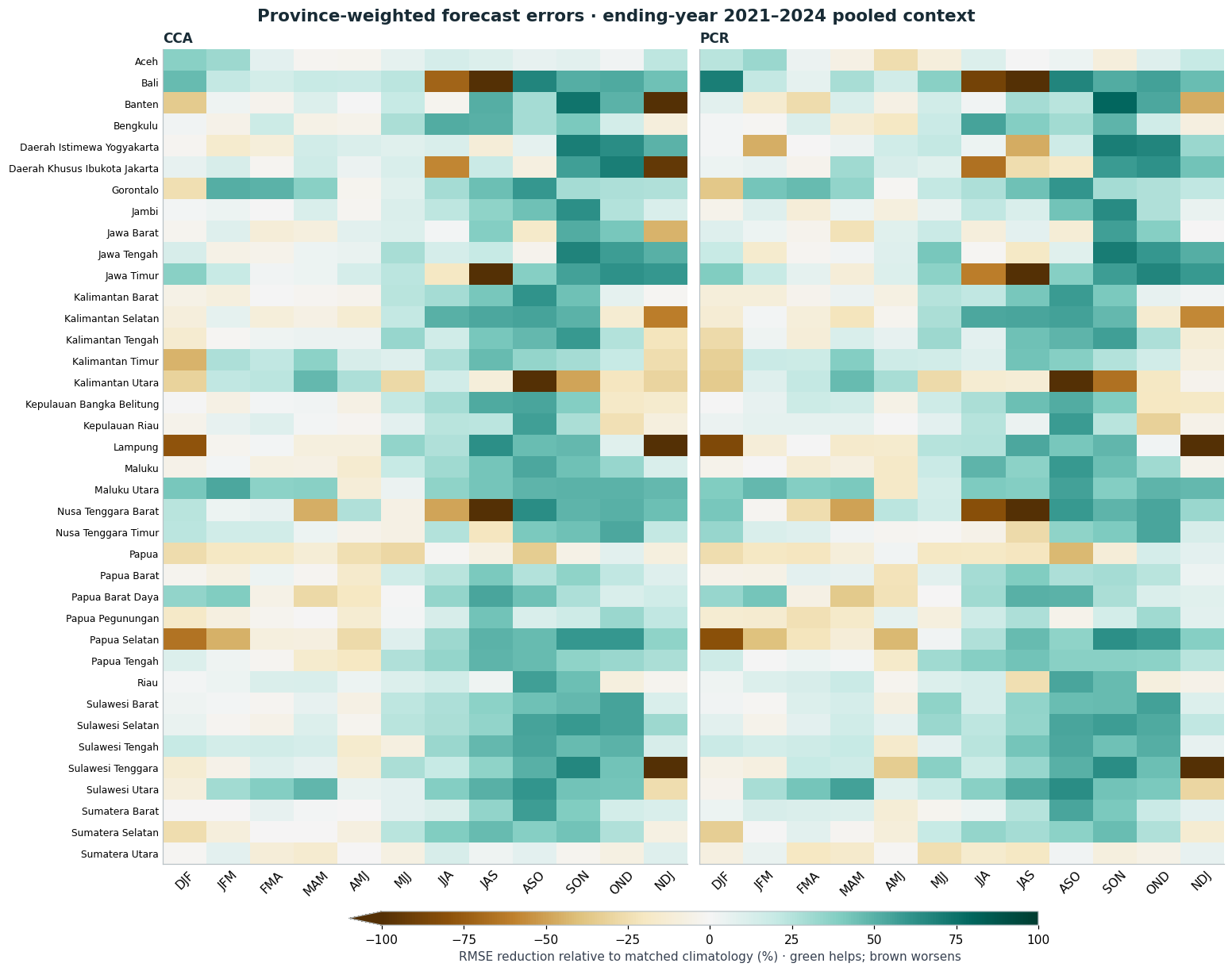
Repeat the comparison using all four original ending-year 2021–2024 labels. Pool annual MSE before taking its square root; each year has equal weight. This context includes2023 and is not independent confirmation of it. It does, however, expose patterns that change when the other archived years are included. Seven forecast variants, both training periods, raw and matched climatologies remain in the downloadable annual and pooled tables.
Figure 17.7: The same provinces and fixed colour scale using pooled ending-year 2021–2024 errors. This includes2023, not an independent validation set. Equal-year MSE is averaged before the square root.
(root /'docs/_includes').mkdir(exist_ok=True)#| label: regional-findingsdef province_win_counts(ds): chosen = ds.sel(region=province_names) base = chosen.rmse.sel(forecast_variant='climatology_1991_2020')return {m: (chosen.rmse.sel(forecast_variant=f'{m.lower()}_1991_2020') < base).sum('region').to_pandas().reindex(teach.SEASONS) for m in ('CCA','PCR')}counts23 = province_win_counts(regional)counts4 = province_win_counts(regional_pooled)province_counts = pd.DataFrame({'2023 CCA':counts23['CCA'], '2023 PCR':counts23['PCR'],'Four-year CCA':counts4['CCA'], 'Four-year PCR':counts4['PCR']})province_counts.index.name ='Season'province_counts.to_csv(artifacts /'province-improvement-counts.csv')display(HTML(province_counts.to_html(classes='table table-sm', border=0)))regional_summary = {'provinces':38, 'unassigned_weight_percent':100*unassigned_fraction,'native_points':region_provenance['native_points'], 'unassigned_points':region_provenance['unassigned_points'],'overlap_points':region_provenance['overlap_points'], 'province_counts':province_counts.to_dict(),'scope':'Descriptive province-weighted coarse-cell errors; overlapping seasons and four years do not establish operational skill'}(artifacts /'regional-findings.json').write_text(json.dumps(regional_summary, indent=2)+'\n')regional_text = (f"For OND 2023, CCA has lower RMSE than climatology in **{int(counts23['CCA']['OND'])} of 38 provinces**, "f"and PCR in **{int(counts23['PCR']['OND'])} of 38**. For JJA 2023, the corresponding counts are "f"**{int(counts23['CCA']['JJA'])}** and **{int(counts23['PCR']['JJA'])}**, despite the national comparison favouring climatology. "f"In the four-year pooled JJA context, they become **{int(counts4['CCA']['JJA'])}** and **{int(counts4['PCR']['JJA'])}**. ""Those changes show why one year should not be turned into a province-specific forecast recommendation.")small = support_table[support_table['Region'].isin(province_names)].sort_values('Contributing coarse cells').iloc[0]regional_text += (f" The smallest support is **{small['Region']}**, with **{int(small['Contributing coarse cells'])} coarse cells**; "f"its largest single cell carries **{small['Largest single-cell share (%)']:.1f}%** of its weight. These are support diagnostics, not independent sample counts.")(root /'docs/_includes/regional-findings.qmd').write_text(regional_text+'\n')coverage_text = (f"The province polygons contain **{100*(1-unassigned_fraction):.2f}%** of the original country weight. "f"The remaining **{100*unassigned_fraction:.2f}%** ({region_provenance['unassigned_points']:,} native country pixels) ""is retained as an explicit unassigned category. There are no multiply assigned native pixels. ""Province plus residual errors recombine to the unchanged national scores.")(root /'docs/_includes/regional-coverage.qmd').write_text(coverage_text+'\n')print('Regional findings and all-season count table exported; counts are descriptive, not independent samples.')
2023 CCA
2023 PCR
Four-year CCA
Four-year PCR
Season
DJF
19
20
17
21
JFM
21
15
23
23
FMA
22
14
22
22
MAM
20
20
22
24
AMJ
25
25
13
15
MJJ
22
25
32
30
JJA
8
8
32
28
JAS
17
14
31
27
ASO
34
34
33
33
SON
32
33
35
34
OND
32
31
32
32
NDJ
21
20
21
23
Regional findings and all-season count table exported; counts are descriptive, not independent samples.
8. Keep the training-period sensitivity visible
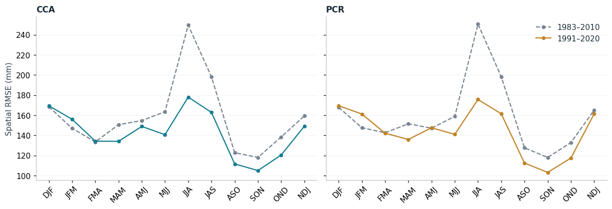
Compare the same forecast windows using 1983–2010 (28 training seasons) and 1991–2020 (30). The common older start avoids missing 1981 initializations for the cross-year seasons in the original all-season design. This changes training years, sample count, EOF bases and fitted relationships together. It is not a controlled estimate of the effect of sample count alone, and does not justify selecting whichever period happens to win a particular 2023 season.
sensitivity = rmse[[f"{m}_{p}"for m in ("climatology", "cca", "pcr") for p in ("1983_2010", "1991_2020")]]sensitivity.to_csv(artifacts /"training-period-sensitivity.csv")fig = teach.sensitivity_plot(rmse)teach.save_figure(fig, artifacts, "training-sensitivity")plt.show()
Figure 17.8: The same target windows with two fixed training intervals. Both sample count and training years change; this is a sensitivity comparison, not a period-selection rule.
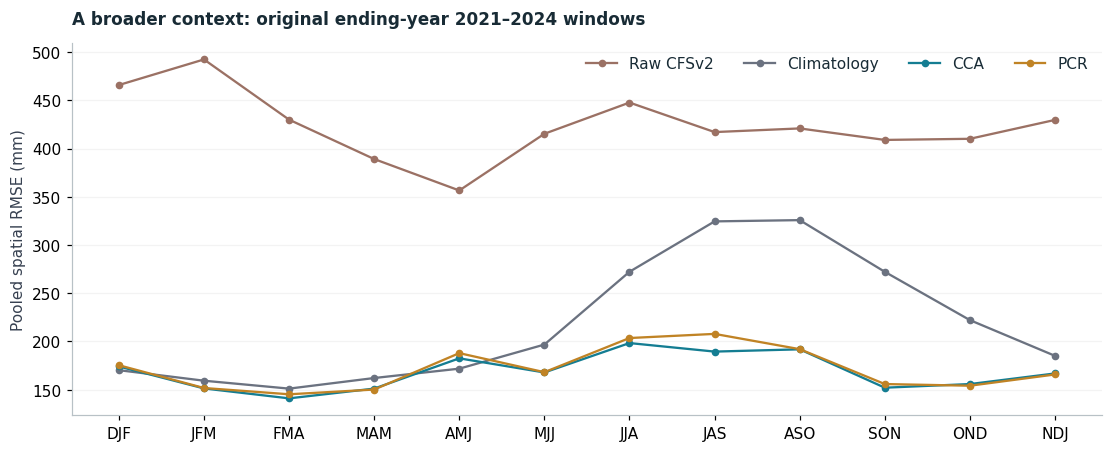
The original benchmark covers ending-year labels 2021–2024. Retain that convention here: its NDJ windows are November 2020–January 2021 through November 2023–January 2024. This is not four complete midpoint-calendar-year collections. The 2023-centred selection above uses the final NDJ window.
Pooled RMSE takes the square root after averaging squared errors across years and locations; it is not the arithmetic mean of annual RMSE. The assertions below check that identity with equal annual coverage. Four years, overlapping seasons and spatially correlated cells do not establish general operational forecast skill.
Figure 17.9: Pooled spatial errors in the original ending-year 2021–2024 benchmark. These labels differ from the midpoint-year selection used for the main 2023 case.
10. Export findings for the story and check provenance
The story includes the following generated text. Its numerical claims come from the same scores used in the figures, so a revised execution cannot silently leave manually copied numbers in the narrative. The final hash check confirms that none of the packaged inputs changed during execution.
wins = {m: int((main_rmse[m] < main_rmse["Climatology"]).sum()) for m in ("CCA", "PCR")}raw_wins = {m: int((main_rmse[m] < main_rmse["Raw CFSv2"]).sum()) for m in ("CCA", "PCR")}best = main_rmse.idxmin(axis=1)climo_best = best.index[best =="Climatology"].tolist()ond = main_rmse.loc["OND"]period_wins = {m: int((rmse[f"{m}_1991_2020"] < rmse[f"{m}_1983_2010"]).sum()) for m in ("cca", "pcr")}summary = {"main_year_convention": "Midpoints in2023; NDJ source ending-year2024", "main_training_period": "1991–2020","calibration_beats_climatology_seasons": wins, "calibration_beats_raw_seasons": raw_wins,"lowest_rmse_method_by_season": best.to_dict(), "ond_rmse_mm": ond.to_dict(),"recent_training_lower_rmse_seasons": period_wins,"original_context_pooled_rmse_mm": context_table.to_dict(), "data_input_hashes": provenance["outputs"]}(artifacts /"findings.json").write_text(json.dumps(summary, indent=2) +"\n")text = (f"Across the twelve windows centred on 2023, CCA reduced spatial RMSE relative to the raw model in **{raw_wins['CCA']} seasons**; "f"PCR did so in **{raw_wins['PCR']}**. Against the more demanding climatology baseline, CCA improved in **{wins['CCA']} of 12** "f"and PCR in **{wins['PCR']} of 12**.\n\n"+ (f"Climatology had the lowest RMSE of all four methods in **{', '.join(climo_best)}**. "if climo_best else"Climatology was not the lowest-RMSE method in this particular set of windows. ")+"These are descriptive comparisons for these forecast windows, not a test of statistical significance.")includes = root /"docs/_includes"includes.mkdir(exist_ok=True)(includes /"seasonal-findings.qmd").write_text(text +"\n")ond_text = (f"For OND, spatial RMSE was **{ond['Raw CFSv2']:.1f} mm** for the raw model and **{ond['Climatology']:.1f} mm** for climatology, "f"compared with **{ond['CCA']:.1f} mm** for CCA and **{ond['PCR']:.1f} mm** for PCR. ""Those numbers describe errors over country-land cells; they are not national-mean rainfall totals.")(includes /"ond-findings.qmd").write_text(ond_text +"\n")teach.verify_bundle(data_dir)display(HTML(f"<p><strong>Input integrity passed.</strong> CCA beats climatology in {wins['CCA']}/12 seasons; PCR in {wins['PCR']}/12.</p>"))
Input integrity passed. CCA beats climatology in 9/12 seasons; PCR in 7/12.
What this notebook does not establish
The twelve windows overlap; they are not twelve independent annual samples. The reference observations and archived model fields use current data vintages, not an exact reconstruction of everything available when forecasts were issued. The CFSv2 archive appends operational forecasts from April 2011; continuity does not establish homogeneity. Physical EOF/CCA-pattern review, independent station checks, longer validation and predefined regional diagnostics remain follow-up work.
Native probabilities are deliberately outside this first comparison. Their category reference dates differ from some training periods; zero-bounded outputs do not always equal their unbounded locations. Some high-level notebook probability scores are in-sample, and flexible exceedance calculations differ from native CPT17. Read the book’s methods and limitations page before using those outputs.
Saha, S., Moorthi, S., Wu, X., et al. (2014). The NCEP Climate Forecast System Version 2. Journal of Climate, 27(6), 2185-2208. https://doi.org/10.1175/JCLI-D-12-00823.1
Kirtman, B., Min, D., Infanti, J., et al. (2014). The North American Multimodel Ensemble: Phase-1 seasonal-to-interannual prediction; Phase-2 toward developing intraseasonal prediction. Bulletin of the American Meteorological Society, 95(4), 585-601. https://doi.org/10.1175/BAMS-D-12-00050.1
Climate Hazards Center, UC Santa Barbara. CHIRPS: Rainfall Estimates from Rain Gauge and Satellite Observations (CHIRPS version 3.0 page). https://www.chc.ucsb.edu/data/chirps3
Funk, C., Peterson, P., Landsfeld, M., et al. (2014). A quasi-global precipitation time series for drought monitoring. U.S. Geological Survey Data Series 832. https://doi.org/10.3133/ds832