Twelve seasons over Indonesia

When calibration helped rainfall forecasts centred on 2023, and when climatology did better

import {selectControl, nationalHeatmap, gainBars, rainfallMaps, errorMaps, provinceView, sensitivity, nationalContext} from "../assets/story/story.js"
storyData = FileAttachment("../assets/story/metrics.json").json()
trainingOptions = [["1991_2020", "1991–2020 (main)"], ["1983_2010", "1983–2010 (sensitivity)"]]
mapFiles = ({fields: FileAttachment("../assets/story/fields.json").url(),
  indonesia: FileAttachment("../data/boundaries/indonesia.geojson").url(),
  provinces: FileAttachment("../data/boundaries/provinces.geojson").url(),
  neighbours: FileAttachment("../data/boundaries/neighbours.geojson").url()})

Seasonal rainfall · Indonesia · 0.25° observation grid

Imagine receiving a rainfall forecast for October to December. A map full of detail tells you where the model expects rain. It does not tell you whether those details are useful. For that, the forecast needs to face an observation reference and an alternative that asks very little of the model: the average rainfall observed in previous years.

Here we make that comparison across twelve seasons. Each is a three-month window, shifted forward by one month, with its midpoint in 2023. The question is whether statistical calibration improves the raw forecast, whether it also improves on climatology, and how the answer changes across seasons and locations.

Hover or tap a figure to inspect its values. The controls let you explore other seasons, score types and provinces; the story’s main comparison remains 1991–2020. Use Download current view (PNG) to save a figure with your selections and its legend. Charts also offer Download current view (SVG) for scalable vector figures with editable text. Notebook reference PNG links open the original executed figures; their labels identify the metric or coverage they contain. Expandable data tables provide numeric downloads.

NoteThe short result

Across the twelve windows centred on 2023, CCA reduced spatial RMSE relative to the raw model in 12 seasons; PCR did so in 12. Against the more demanding climatology baseline, CCA improved in 9 of 12 and PCR in 7 of 12.

Climatology had the lowest RMSE of all four methods in DJF, JJA, JAS. These are descriptive comparisons for these forecast windows, not a test of statistical significance.

Four ways to forecast the same rainfall

All four methods are evaluated against the same CHIRPS3 rainfall totals on the same 3,240 country-land grid cells. The raw forecast is the CFSv2 ensemble mean, supplied at 1° and interpolated to the observation grid. Climatology predicts the observed training-period average for each place and season.

PCR and CCA learn relationships between model rainfall patterns and observed rainfall. PCR compresses the predictor field into a small set of components before regression. CCA also compresses the observation field and relates the two sets of patterns. The IRI teaching reference introduces both approaches and the role of cross-validation.

For this illustration, the calibrated models use 1991–2020 training data. They retain fixed, small mode counts: three predictor EOFs for both methods, and three predictand EOFs plus two CCA modes for CCA. These counts were held fixed across the experiment; they are not claimed to be optimal for Indonesia.

The forecasts are evaluated over full Indonesia, rather than a selection of locations where calibration happened to work. The 0.25° grid describes the observation aggregation and forecast output. It does not establish that the dynamical model predicts rainfall independently at that spatial resolution.

A year needs a careful calendar

DJF in this story means December 2022–February 2023. At the other end of the sequence, NDJ means November 2023–January 2024. That final window is stored as NDJ 2024 in the research files, because those files label seasons by their ending year. We preserve that label and show actual dates in the notebook.

Each forecast is initialized one month before its target begins. This holds the lead design consistent across seasons. These are archived historical forecasts, verified later against current-vintage observations, not a reconstruction of every data product exactly as it existed on the original issue date.

ImportantTwelve windows are not twelve independent years

Adjacent seasons share two months. Counting more overlapping windows does not turn this one-year case study into twelve independent annual validation samples.

Start with the national comparison

The chart measures spatial error across the country. Lower RMSE means smaller errors, with larger local errors receiving more weight. It is not the error of a single national-mean rainfall value. Every method uses identical observed totals and country-land weights.

viewof nationalMetric = selectControl("National score", [["rmse", "RMSE"], ["mae", "MAE"], ["bias", "Bias"]], "rmse")
nationalHeatmap(storyData, nationalMetric)

National forecast scores across twelve seasons.

Notebook reference PNG (RMSE) · Executed notebook figure

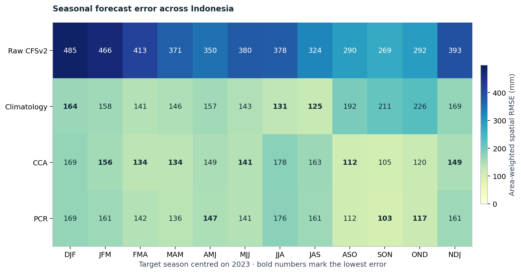
The first benchmark asks whether calibration improves on the raw model. The second asks whether it beats climatology. These are different hurdles. A model can become much less biased after calibration yet still offer little advantage over the historical average for a particular season.

The next chart makes the second comparison explicit. Values below zero favour climatology. Small positive differences deserve the same caution as small negative ones: this experiment reports their size, without assigning statistical significance to them.

viewof gainPeriod = selectControl("Calibration period for reduction chart", trainingOptions, "1991_2020")
gainBars(storyData, gainPeriod)

RMSE reduction against the selected training-period climatology. Positive is better.

Notebook reference PNG (1991–2020) · Executed notebook figure

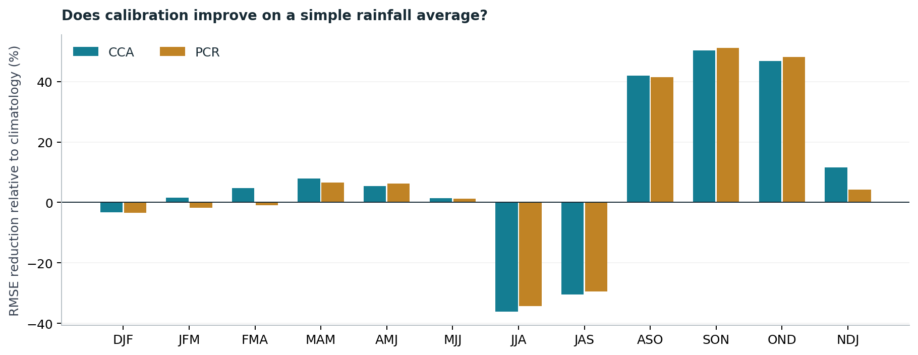
For the main 2023 selection, DJF, JJA and JAS are reminders to keep the simple baseline in view. Neither calibrated method has the lowest national RMSE there. That finding would disappear from a tutorial restricted to a successful OND example.

Work through OND

OND is a useful place to examine the workflow in detail. A forecast initialized on 1 September 2023 is compared with accumulated rainfall from 1 October to 31 December. In the notebook, the exact training inputs are loaded, their dates are checked, and their observed average is compared with the saved climatology. An optional cell shows the CCA and PCR calls and can rerun them in new scratch directories in the tested PyCPT fitting environment. Reading the executed notebook or running its default saved-results analysis needs no PyCPT/CPT installation or IRI Data Library key; the requirements guide explains the distinction.

viewof rainfallSeason = selectControl("Rainfall map season", storyData.seasons, "OND")
viewof rainfallPeriod = selectControl("Rainfall map training period", trainingOptions, "1991_2020")
rainfallPlot = {
  const view = rainfallMaps(storyData, mapFiles, rainfallSeason, rainfallPeriod);
  invalidation.then(() => view.dispose());
  return view;
}

Start with OND, then explore the other windows. The five maps always use one common rainfall scale for the selected season.

Notebook reference PNG (OND 2023; 1991–2020) · Executed notebook figure

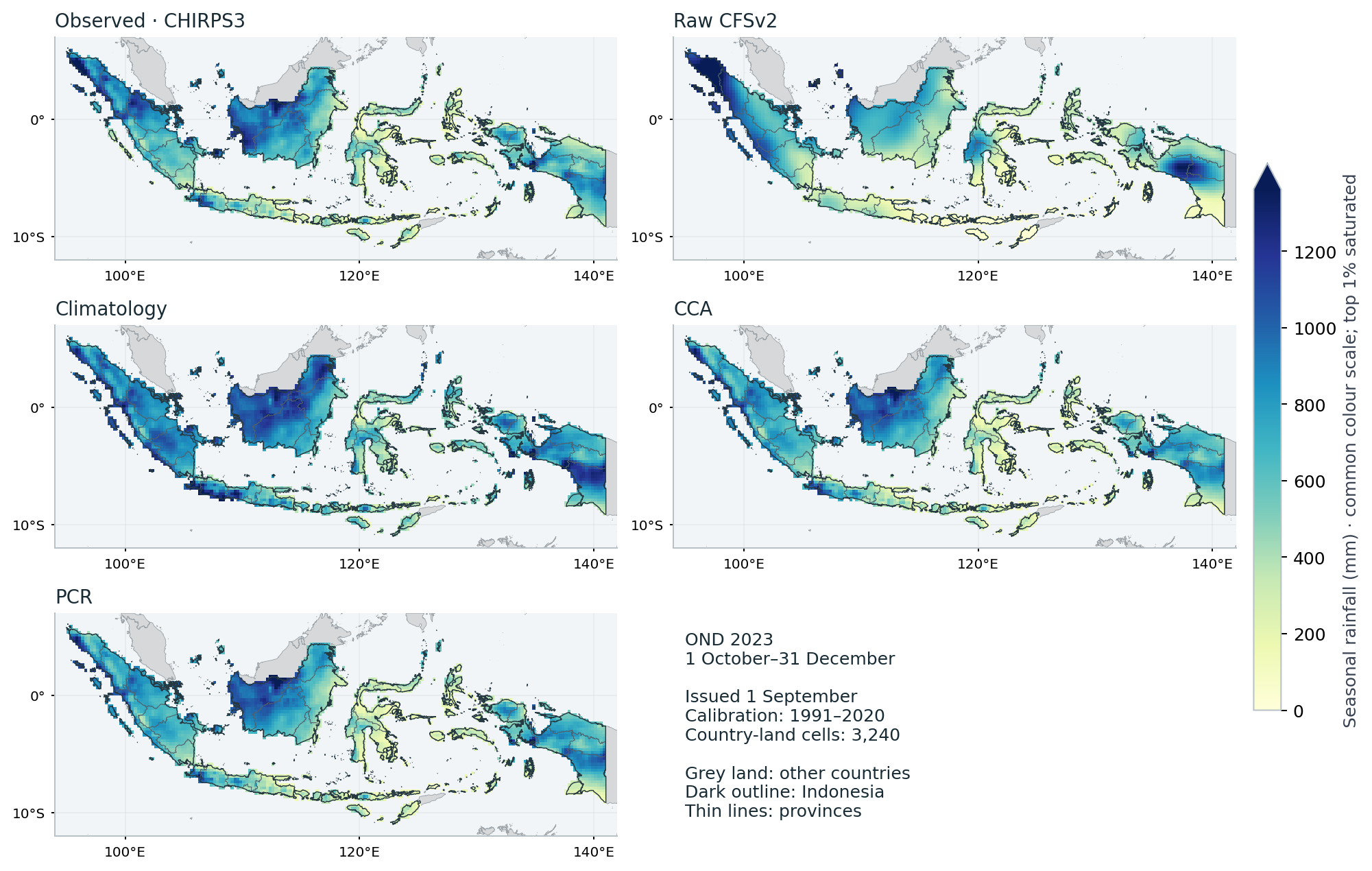
For OND, spatial RMSE was 292.4 mm for the raw model and 226.5 mm for climatology, compared with 120.3 mm for CCA and 117.4 mm for PCR. Those numbers describe errors over country-land cells; they are not national-mean rainfall totals.

Grey land shows other countries. Indonesia is unfilled by the boundary overlay, with a dark country outline and thin province lines over the rainfall fields. These display boundaries do not change the evaluation footprint or scores.

The common map scale helps expose differences between the raw field, the observed reference and the calibrated fields. Inspecting these patterns is useful, but visual resemblance is not the scoring rule. The reported ranking comes from cell-by-cell errors on the shared footprint.

National improvement can hide local deterioration

The map explorer below compares local absolute errors with climatology. Green cells show where calibration reduced the error; brown cells show where the average was closer to the observation. Choose any of the twelve windows or display them together; both CCA and PCR remain available.

viewof errorSeason = selectControl("Local-error map season", [["all", "All twelve seasons"], ...storyData.seasons.map(s => [s,s])], "JJA")
viewof errorPeriod = selectControl("Local-error map training period", trainingOptions, "1991_2020")
errorPlot = {
  const view = errorMaps(storyData, mapFiles, errorSeason, errorPeriod);
  invalidation.then(() => view.dispose());
  return view;
}

Explore both calibrated methods in any season, or show all twelve. Positive local absolute-error reduction favours calibration; colours saturate beyond ±300 mm.

Notebook reference PNG (all 12 seasons; 1991–2020) · Executed notebook figure

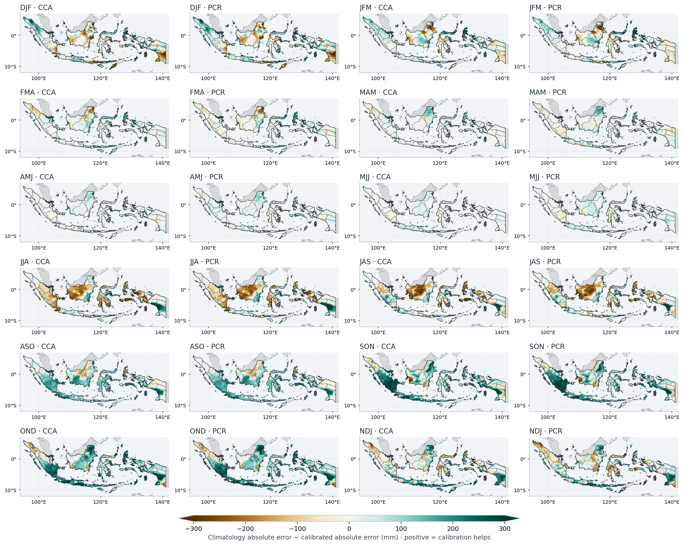
A favourable national score does not mean every island or district benefited. It would be premature to translate these maps directly into recommendations for planting, drought response or rainfall onset.

Do the provinces tell the same story?

We now summarize the same cell errors for all 38 supplied provinces, using unchanged model forecasts. The analysis assigns original country-native 0.05° pixel centres to the unsimplified province polygons and sums their area-weight shares within each existing 0.25° cell. It uses no province-specific fitting or selection of favourable locations.

The province polygons contain 98.69% of the original country weight. The remaining 1.31% (803 native country pixels) is retained as an explicit unassigned category. There are no multiply assigned native pixels. Province plus residual errors recombine to the unchanged national scores.

viewof provinceRegion = selectControl("Province", [["all", "All 38 provinces"], ...storyData.support.filter(r => r.isProvince).map(r => [r.name,r.name]).sort((a,b) => a[0].localeCompare(b[0]))], "all")
viewof provincePeriod = selectControl("Province training period", trainingOptions, "1991_2020")
provinceView(storyData, provinceRegion, provincePeriod, false)

All 38 provinces are included. Choose one province for a four-method seasonal comparison. These are province-weighted views of existing 0.25° cell errors.

Notebook reference PNG (all 38 provinces; 1991–2020) · Executed notebook figure

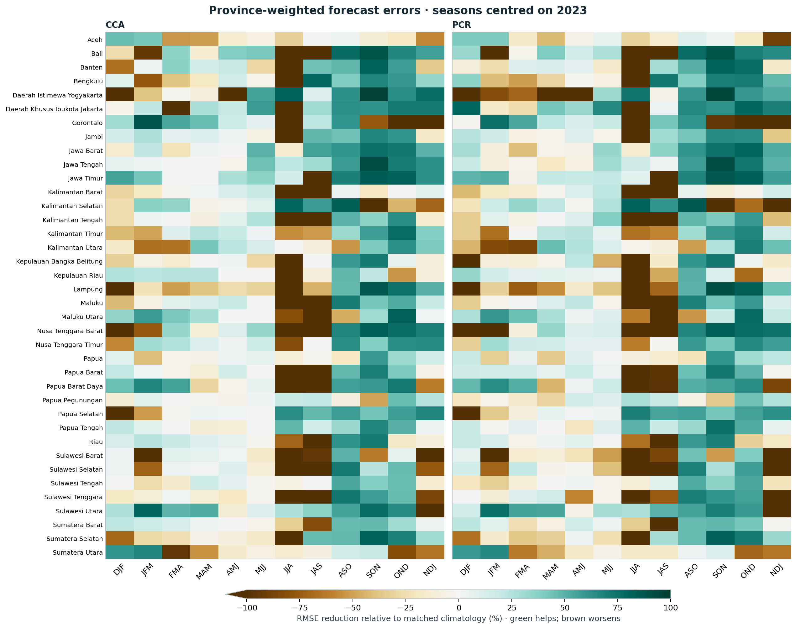
Each province gets its own normalized weights, so small and large provinces can be compared against their own climatology. The colour scale shows relative error reduction; the numeric downloads retain RMSE, MAE and bias for both training periods, the raw model and matched climatologies.

For OND 2023, CCA has lower RMSE than climatology in 32 of 38 provinces, and PCR in 31 of 38. For JJA 2023, the corresponding counts are 8 and 8, despite the national comparison favouring climatology. In the four-year pooled JJA context, they become 32 and 28. Those changes show why one year should not be turned into a province-specific forecast recommendation. The smallest support is Daerah Khusus Ibukota Jakarta, with 3 coarse cells; its largest single cell carries 63.2% of its weight. These are support diagnostics, not independent sample counts.

provinceView(storyData, provinceRegion, provincePeriod, true)

Original ending-year 2021–2024 pooled context, including 2023. This view follows the province and training-period controls above.

Notebook reference PNG (all 38 provinces; 1991–2020) · Executed notebook figure

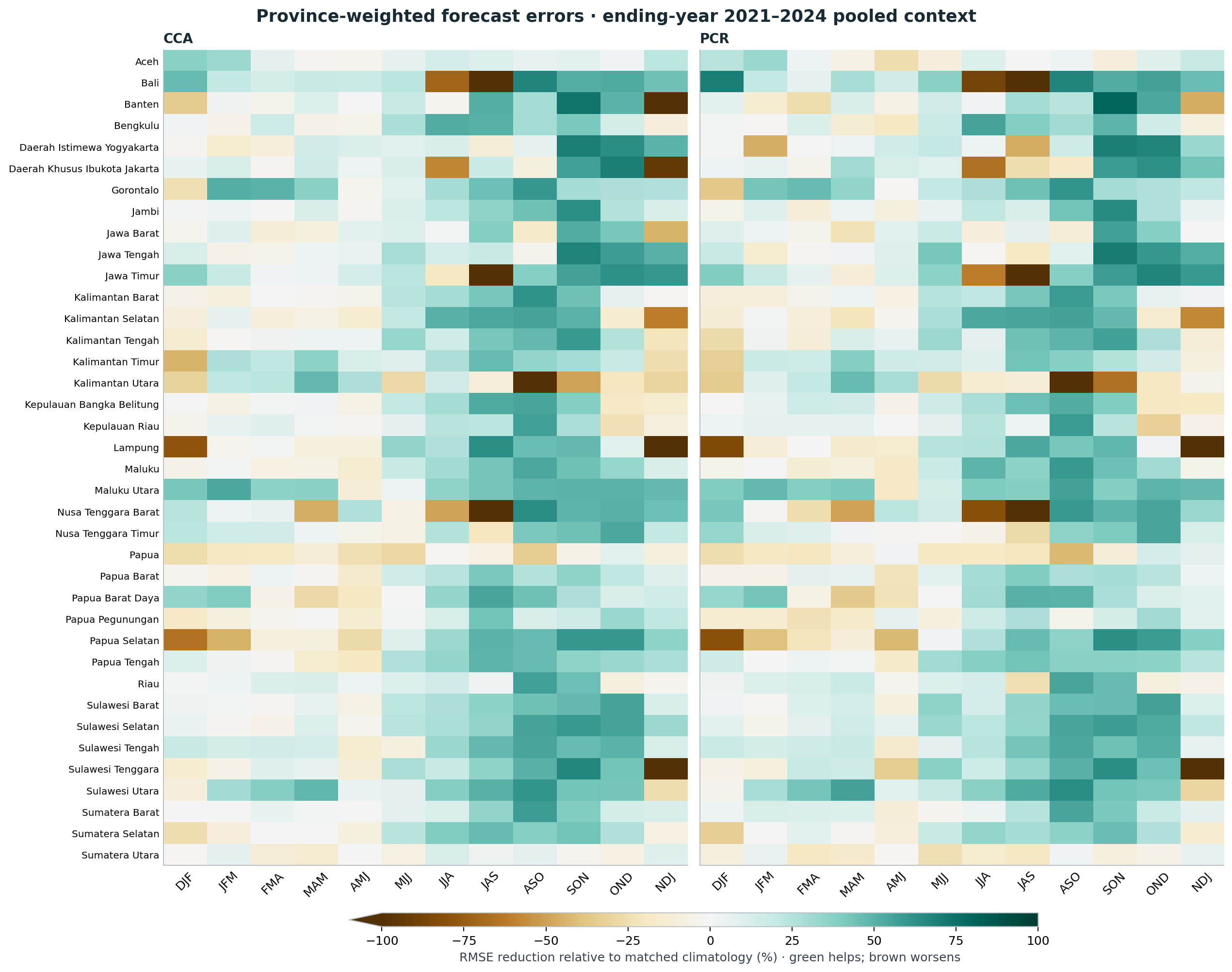
The second figure adds the original ending-year 2021–2024 context, including 2023. It is not an independent validation set. A green cell in one year does not establish stable provincial forecast skill.

These are province-weighted views of coarse-cell errors. A grid cell shared by two provinces retains the same forecast and observation error in both, with different weight shares. This does not resolve province-only rainfall inside the cell. The notebook reports cell support and the largest single-cell weight share, which matter especially for small provinces, alongside an assignment audit map. See the regional provenance and province scores, or the four-method OND table.

How much depends on the training period?

We also keep the 1983–2010 fits. Comparing them with 1991–2020 changes the sample count as well as the years and fitted patterns. It is a sensitivity experiment, not a rule to choose whichever period happens to give the most attractive map for a particular season.

viewof sensitivityMethod = selectControl("Method for period comparison", ["CCA", "PCR"], "CCA")
sensitivity(storyData, sensitivityMethod)

Compare fixed training intervals for the same targets. Changing the interval changes both sample count and fitted relationships.

Notebook reference PNG (CCA and PCR) · Executed notebook figure

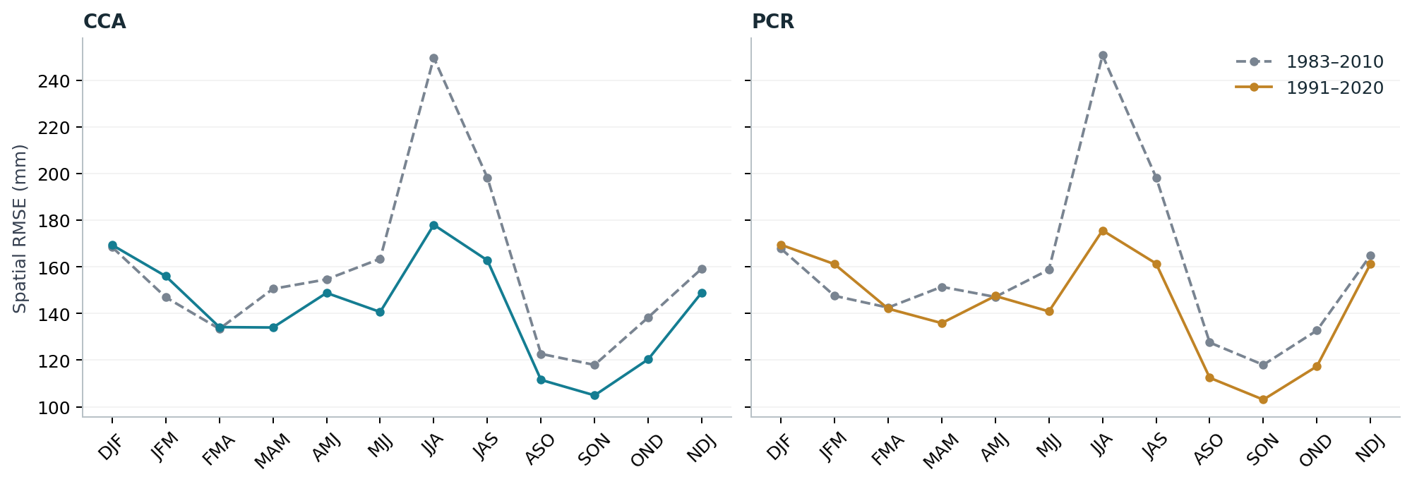
The older interval starts in 1983 so that every season has a common set of available initializations. This is a design choice, not a universal CPT training period. Climatology baselines are calculated from each fit’s own training years.

Look beyond this one selection

The original research benchmark contains four ending-year labels, 2021–2024. Its pooled comparison provides context for the 2023 case and shows whether the same broad conclusions persist across more than one target year.

viewof contextMetric = selectControl("Pooled context score", [["rmse", "RMSE"], ["mae", "MAE"], ["bias", "Bias"]], "rmse")
nationalContext(storyData, contextMetric)

Pooled scores retain the original ending-year 2021–2024 labels. Equal-year MSE precedes the square root for RMSE.

Notebook reference PNG (RMSE; 1991–2020) · Executed notebook figure

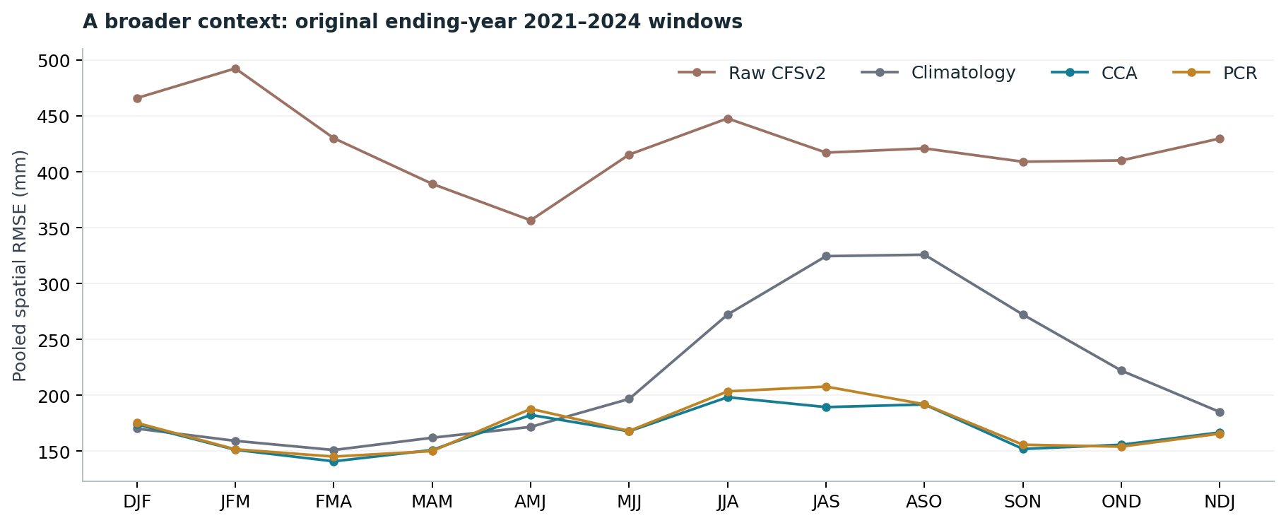
Here the year convention is the original one: for NDJ, the four windows run from November 2020–January 2021 through November 2023–January 2024. This is not four complete collections of seasons centred on calendar years. AMJ climatology remains competitive in this broader comparison even though the main 2023 selection favours calibration there. That difference is a reason to retain the broader context rather than treating one year as a forecast-system verdict.

What this first study supports

Calibration can substantially change the errors in these historical forecasts, and its value depends on season, location, baseline and training interval. A useful tutorial should show those dependencies and the cases where calibration does not win.

This study does not establish general operational skill or probability reliability. It uses gridded observations, a mixed reforecast/operational model archive and only a few verification years. Longer independent validation, regional diagnostics and physical interpretation of the fitted patterns remain necessary before a recommended forecasting configuration.

Continue with the executed notebook, the reproduction guide, or the methods and limitations. The notebook exports the numeric scores, calendar, and computed findings behind this story.

References

1. IRI. Guide to PyCPT 2 for Seasonal Climate Forecasts (Jupyter Book, 2 September 2023 build): The Climate Predictability Tool (CPT). https://iri.columbia.edu/~awr/pycpt/seasonal-jupyterbook/html_2sep2023/cpt.html
2. IRI. CPT+: Climate Predictability Tool. https://iri.columbia.edu/our-expertise/climate/tools/cpt/
3. IRI Data Library. NMME NCEP-CFSv2 hindcasts, PENTAD_SAMPLES_FULL, precipitation. https://iridl.ldeo.columbia.edu/SOURCES/.Models/.NMME/.NCEP-CFSv2/.HINDCAST/.PENTAD_SAMPLES_FULL/.prec/ Browsing Data Library pages requires signing in (checked 10 November 2026); PyCPT’s data requests in this tutorial succeeded without a key.
4. Saha, S., Moorthi, S., Wu, X., et al. (2014). The NCEP Climate Forecast System Version 2. Journal of Climate, 27(6), 2185-2208. https://doi.org/10.1175/JCLI-D-12-00823.1
5. Kirtman, B., Min, D., Infanti, J., et al. (2014). The North American Multimodel Ensemble: Phase-1 seasonal-to-interannual prediction; Phase-2 toward developing intraseasonal prediction. Bulletin of the American Meteorological Society, 95(4), 585-601. https://doi.org/10.1175/BAMS-D-12-00050.1
6. Climate Hazards Center, UC Santa Barbara. CHIRPS: Rainfall Estimates from Rain Gauge and Satellite Observations (CHIRPS version 3.0 page). https://www.chc.ucsb.edu/data/chirps3
7. Funk, C., Peterson, P., Landsfeld, M., et al. (2014). A quasi-global precipitation time series for drought monitoring. U.S. Geological Survey Data Series 832. https://doi.org/10.3133/ds832