Folders, the forecast question and the two settings dictionaries
This chapter starts the PyCPT workflow that the rest of Learn PyCPT builds on. By the end you will have a case folder, a complete description of the forecast you want to calibrate, and a map of the two domains. Nothing is downloaded from the IRI Data Library yet, so no account or key is needed.
The running example: CFSv2 rainfall forecasts initialized on 1 September 2023 for October to December (OND) 2023 over Indonesia, trained on the 1991-2020 target seasons. It is the same forecast as the Fit & diagnose case study, so later chapters can check PyCPT’s high-level workflow against those saved results.
The steps follow IRI’s operational seasonal template, the maintained starting point for PyCPT 2.10. Where this page explains behaviour that the template leaves implicit, the explanation comes from the installed PyCPT 2.10.4 source.
NoteWhat you need to run this page
Reading it needs only a browser. Running it needs the full PyCPT environment in Setup & downloads and this tutorial’s repository, which holds the small figure helper used for the map. The map in step 7 fetches Natural Earth coastlines the first time it runs, so that cell needs internet access once.
1. Check the PyCPT version
PyCPT is several Python packages. pycpt holds the high-level workflow used in these chapters; cptdl holds the data catalog and download code. The template refuses to run below PyCPT 2.10.0. A minimum version is a useful guard, but it does not prove that every dataset and argument behaves as it did when a page was written, so we also print the version this page was executed with.
from pathlib import Pathimport datetime as dtimport sysimport textwrapimport matplotlib.pyplot as pltimport packaging.versionimport pandas as pdimport pycptimport cptdl as dlrepo =next((p for p in (Path.cwd(), *Path.cwd().parents) if (p /"pycpt_tutorial").is_dir()), None)sys.path.insert(0, str(repo))from pycpt_tutorial import figuresfigures.use_style()print(f"Installed PyCPT: {pycpt.__version__}")print("This page was executed with the pinned PyCPT 2.10.4 environment.")if packaging.version.parse(pycpt.__version__) < packaging.version.parse("2.10.0"):raiseRuntimeError("These chapters need PyCPT 2.10.0 or newer. See Setup & downloads.")
Installed PyCPT: 2.10.4
This page was executed with the pinned PyCPT 2.10.4 environment.
2. Choose the model and the observations
The catalog is three dictionaries in cptdl: hindcasts, forecasts and observations. Each maps a dataset name to an IRI Data Library URL template. The template notebook’s comment suggests dl.models.keys(); in this version that attribute does not exist, so list dl.hindcasts instead.
rain_models =sorted(name for name in dl.hindcasts if name.endswith(".PRCP"))rain_obs = [name for name in dl.observations if name.endswith(".PRCP")]print(f"{len(dl.hindcasts)} hindcast entries, {len(rain_models)} of them rainfall (.PRCP):")print(textwrap.fill(", ".join(rain_models), width=88))print()print(f"{len(rain_obs)} rainfall observation entries:")print(textwrap.fill(", ".join(rain_obs), width=88))print()print("Rainfall names marked as deprecated, with their replacements:")for old, (new, _doc) in dl.catalog.deprecations.items():if old.endswith(".PRCP"):print(f" {old} -> {new}")
A name in the catalog says what PyCPT can request. It does not say that the model has hindcasts for your initialization month and training years; the next chapter checks that after downloading.
We pick one model, one observation dataset and the calibration method. MOS (model output statistics) is "CCA" or "PCR" in the template. Setting local_predictand_file to None means the observations come from the catalog; chapter 3 replaces them with a local CHIRPS3 file.
MOS ="CCA"predictor_names = ["CFSv2.PRCP"]predictand_name ="UCSB.PRCP"local_predictand_file =None
3. Describe the forecast: download_args
download_args defines which data to fetch: the initialization date, the target season, the training years and two bounding boxes.
fdate: the initialization date. Its year is used only for the forecast file; for hindcasts only the month matters.
target: the season as "Mmm-Mmm", here "Oct-Dec".
target_first_year, target_final_year: the training seasons, labelled by the year of the season’s midpoint. December-February 1999-2000 is the 2000 season.
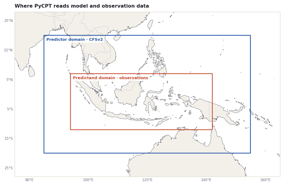
predictor_extent: the model domain, 85°E-155°E and 20°S-20°N. It covers a larger area than the observation box.
predictand_extent: the observation domain, a box around Indonesia.
Both boxes match the Fit & diagnose case. They are a controlled choice, not a recommendation for the best predictor domain.
Before downloading, it helps to see how PyCPT turns these settings into a request. Two conversions happen. The target season becomes a lead range in months after initialization. The training years, given as target years, become initialization years, which differ when the forecast is issued in the calendar year before the season’s midpoint.
The table applies PyCPT’s own helpers to our case and to two cross-year seasons for contrast.
For OND from a September start the leads are 1.5 to 3.5 months and the years do not shift, so training seasons 1991-2020 use September initializations 1991-2020. A December-February forecast issued in November would use initializations from the previous calendar year.
PyCPT does this conversion in an internal function, _preprocess_download_args. We call it here only to show the values it will use; do not build your own code on an underscore-prefixed function. The resolved values fill the URL template, which is the exact recipe sent to the Data Library.
from pycpt import notebook as pycpt_notebookresolved = pycpt_notebook._preprocess_download_args(download_args)for key in ["lead_low", "lead_high", "first_year", "final_year", "filetype"]:print(f"{key:>10}: {resolved[key]}")def show_url(label, template): url = dl.evaluate_url(template, **resolved)print(f"\n{label}:")print(textwrap.fill(url, width=88, break_on_hyphens=False))show_url("CFSv2 hindcasts", dl.hindcasts["CFSv2.PRCP"])show_url("CFSv2 forecast", dl.forecasts["CFSv2.PRCP"])show_url("UCSB observations", dl.observations["UCSB.PRCP"])
Reading the URLs is worth a minute. Each is a chain of Data Library operations, applied left to right:
CFSv2: select September starts (S) and leads 1.5 to 3.5 (L), average over those leads, cut the box, average over ensemble members ([M]average), then multiply by 92, the number of days in OND. The result is an ensemble-mean seasonal total.
The forecast comes from the same Data Library collection as the hindcasts; only the start date changes, to September 2023.
Observations: CHIRPS v2.0 daily data on a 0.25° grid, multiplied by 92 and averaged over each OND season, which again gives a seasonal total.
When results look surprising later, these URLs are the first place to check what was actually requested.
5. Fix the model settings: cpt_args
cpt_args defines how CPT fits the model. The template allows CPT to choose the number of modes within ranges such as (1, 8). Here every range has equal ends, so the mode counts are fixed at the values used in Fit & diagnose. That keeps the comparison in chapter 3 exact. Fixed counts are a teaching control, not a tuned configuration for Indonesia.
Three settings deserve attention now. crossvalidation_window=5 leaves out each training season together with its two neighbours on either side, wrapping at the ends of the period, so a cross-validated hindcast is not fitted on the year it predicts. The Fit & diagnose notebook documents this window for the same CPT 17.8.3 engine. transform_predictand stays None because the template marks transformations as disabled until upstream bugs are fixed. With the masks set to None, every location is fitted and kept.
6. Create the case folder: setup
setup creates a folder for this domain with data, figures and output inside it, and returns its path. The template passes the predictor extent.
case_dir = Path.home() /"PyCPT"/"indonesia-ond-2023-sep-init"domain_dir = pycpt.setup(case_dir, download_args["predictor_extent"])print()print("Domain folder name:", domain_dir.name)print("Contents:", sorted(p.name for p in domain_dir.iterdir()))
Input data will be saved in ~/PyCPT/indonesia-ond-2023-sep-init/85W-155E_to_-20S-20N/data
Figures will be saved in ~/PyCPT/indonesia-ond-2023-sep-init/85W-155E_to_-20S-20N/figures
Output will be saved in ~/PyCPT/indonesia-ond-2023-sep-init/85W-155E_to_-20S-20N/output

Domain folder name: 85W-155E_to_-20S-20N
Contents: ['data', 'figures', 'output']
Two details in that folder are easy to miss.
The folder name uses signed numbers with fixed letters. PyCPT writes {west}W-{east}E_to_{south}S-{north}N. Our name, 85W-155E_to_-20S-20N, therefore means 85°E to 155°E and 20°S to 20°N. Read the numbers, not the letters.
Downloaded files are named by dataset only. The next cell lists the names PyCPT will use for our case.
year = download_args["fdate"].yearplanned = [f"{name}.nc"for name in predictor_names]planned += [f"{name}_f{year}.nc"for name in predictor_names]planned += [f"{predictand_name}.nc"]for name in planned:print(domain_dir /"data"/ name)
None of these names contains the target season, initialization month, training years or predictand domain. In PyCPT 2.10.4 the download helper reuses any existing file with that name unless force_download=True. If you change the season or years but keep the same case folder and set force_download=False, PyCPT will quietly reuse data for the old question.
The safe habit: one case folder per forecast question, as the name indonesia-ond-2023-sep-init does here, and force_download=True whenever you change download_args in an existing folder.
7. Map the domains
A quick map catches swapped signs or a box in the wrong hemisphere before any download. PyCPT’s own check is
which draws the two boxes in two small separate panels. This tutorial draws both boxes on one map with its figure helper, so you can see how they sit together.
The blue box is the predictor (model) domain; the red box is the predictand (observation) domain, where the calibrated forecasts are produced and verified.
What you have now
A version check and the catalog names for one model and one observation dataset.
download_args: the forecast question, with its leads and initialization years checked before any download.
cpt_args: fixed, documented fitting choices.
A case folder, and two habits that prevent silent mistakes: read the folder name’s numbers, and keep one case folder per forecast question.
The next chapter downloads the hindcasts, forecast and observations into this folder and checks which years actually arrived.
Saha, S., Moorthi, S., Wu, X., et al. (2014). The NCEP Climate Forecast System Version 2. Journal of Climate, 27(6), 2185-2208. https://doi.org/10.1175/JCLI-D-12-00823.1
Kirtman, B., Min, D., Infanti, J., et al. (2014). The North American Multimodel Ensemble: Phase-1 seasonal-to-interannual prediction; Phase-2 toward developing intraseasonal prediction. Bulletin of the American Meteorological Society, 95(4), 585-601. https://doi.org/10.1175/BAMS-D-12-00050.1
IRI Data Library. UCSB CHIRPS version 2.0. https://iridl.ldeo.columbia.edu/SOURCES/.UCSB/.CHIRPS/.v2p0/ Browsing Data Library pages requires signing in (checked 10 November 2026); PyCPT’s data requests in this tutorial succeeded without a key.
Funk, C., Peterson, P., Landsfeld, M., et al. (2015). The climate hazards infrared precipitation with stations: a new environmental record for monitoring extremes. Scientific Data, 2, 150066. https://doi.org/10.1038/sdata.2015.66