Download hindcasts, the forecast and observations, then check what arrived
This chapter downloads the three datasets that the first chapter described: CFSv2 hindcasts for September starts 1991-2020, the CFSv2 forecast started on 1 September 2023, and observed OND rainfall from the catalog entry UCSB.PRCP. Then it checks what arrived: which years, which grid, which units and which values.
Every number on this page comes from the executed cells below.
NoteWhat you need to run this page
The full PyCPT environment and internet access to the IRI Data Library. The download time depends on the Data Library server and your connection; it is printed when the cell runs. The comparison in step 7 also reads saved files from this tutorial’s repository and is skipped if they are not present.
1. Repeat the case settings
Each chapter is a separate notebook, so the settings from chapter 1 are repeated here unchanged. force_download=True makes PyCPT fetch fresh copies even if files with the same names exist; chapter 1 showed why that matters.
from contextlib import redirect_stdoutfrom pathlib import Pathimport datetime as dtimport inspectimport ioimport sysimport timeimport matplotlib.pyplot as pltimport numpy as npimport pandas as pdimport xarray as xrimport cptdl as dlimport pycptfrom pycpt import notebook as pycpt_notebooktutorial_root =next((p for p in (Path.cwd(), *Path.cwd().parents) if (p /"pycpt_tutorial").is_dir()), None)sys.path.insert(0, str(tutorial_root))from pycpt_tutorial import figuresfigures.use_style()MOS ="CCA"predictor_names = ["CFSv2.PRCP"]predictand_name ="UCSB.PRCP"local_predictand_file =Nonedownload_args = {"fdate": dt.datetime(2023, 9, 1),"target": "Oct-Dec","target_first_year": 1991,"target_final_year": 2020,"predictor_extent": {"west": 85, "east": 155, "south": -20, "north": 20},"predictand_extent": {"west": 94, "east": 142, "south": -12, "north": 7},}force_download =Truecase_dir = Path.home() /"PyCPT"/"indonesia-ond-2023-sep-init"domain_dir = pycpt.setup(case_dir, download_args["predictor_extent"])
Input data will be saved in ~/PyCPT/indonesia-ond-2023-sep-init/85W-155E_to_-20S-20N/data
Figures will be saved in ~/PyCPT/indonesia-ond-2023-sep-init/85W-155E_to_-20S-20N/figures
Output will be saved in ~/PyCPT/indonesia-ond-2023-sep-init/85W-155E_to_-20S-20N/output
2. Does this download use your IRI key?
The authentication guide explains that some Data Library datasets require a key. Whether a particular call sends one is a question about the code, so we read it. In PyCPT 2.10.4, download_data reaches the network through cached_download, which calls cptdl.download; that function forwards use_dlauth to simple_download, which attaches the key cookie only when use_dlauth is True. The cell prints those lines from the installed source.
def show_lines(function, words): source = inspect.getsource(function).splitlines()print(f"--- {function.__module__}.{function.__name__}")for number, line inenumerate(source, start=1):ifany(word in line for word in words):print(f"{number:4d} | {line}")show_lines(pycpt_notebook.cached_download, ["dl.download(", "force_download"])show_lines(dl.download, ["def download", "simple_download("])show_lines(dl.simple_download, ["def simple_download", "use_dlauth", "cookies"])
--- pycpt.notebook.cached_download
   1 | def cached_download(url_pattern, files_root, basename, force_download, download_args):
   6 |     if not ncfile.is_file() or force_download:
   8 |         ds = dl.download(
--- cptdl.utilities.download
   1 | def download(baseurl, dest, verbose=False, use_dlauth=False, **kwargs):
  12 |     path = simple_download(url, dest, verbose=verbose, use_dlauth=use_dlauth)
--- cptdl.utilities.simple_download
   1 | def simple_download(url, dest, verbose=False, use_dlauth=False):
   4 |     if str(use_dlauth) == 'True':
   6 |         assert dlauthid is not None, "You need to use cpttools.setup_dlauth('your_email') to get a cookie before you can download this data! or, you can try setting use_dlauth=False"
   7 |         cookies = {'__dlauth_id': dlauthid}
   9 |         cookies={}
  10 |     with requests.post(url, stream=True, allow_redirects=True, cookies=cookies) as r:
cached_download passes no use_dlauth argument, so the default False applies and no cookie is sent. To confirm this at run time, the next cell counts attempts to open any file whose name contains dlauth, the name PyCPT uses for the stored key. It only counts; it never reads a file.
credential_file_opens = {"count": 0}def count_credential_opens(event, args):if event =="open"andisinstance(args[0], (str, bytes)) and"dlauth"instr(args[0]).lower(): credential_file_opens["count"] +=1sys.addaudithook(count_credential_opens)print("Counting credential-file opens from here on.")
Counting credential-file opens from here on.
3. Download
download_data returns three things: the observations Y, a list of hindcast arrays (one per model) and a list of forecast arrays. PyCPT prints the URL of each request and a progress bar. The cell keeps the URLs and drops the progress bars, which are only screen updates.
log = io.StringIO()start = time.monotonic()with redirect_stdout(log): Y, hindcast_data, forecast_data = pycpt.download_data( predictand_name, local_predictand_file, predictor_names, download_args, domain_dir, force_download)elapsed = time.monotonic() - startfor line in log.getvalue().replace("\r", "\n").splitlines():if line.strip() andnot line.startswith("DOWNLOADING:"):print(line)print(f"\nDownload time: {elapsed:.0f} s")print("Credential-file opens during the download:", credential_file_opens["count"])
Downloading CFSv2.PRCP_f2023
URL: https://iridl.ldeo.columbia.edu/SOURCES/.Models/.NMME/.NCEP-CFSv2/.HINDCAST/.PENTAD_SAMPLES_FULL/.prec/S/%280000%201%20Sep%202023%29/VALUES/L/1.5/3.5/RANGEEDGES/%5BL%5D//keepgrids/average/Y/-20/20/RANGEEDGES/X/85/155/RANGEEDGES/%5BM%5D/average/92/mul/-999/setmissing_value/%5BX/Y%5D%5BL/S/add%5D/cptv10.tsv
Downloading UCSB.PRCP
URL: https://iridl.ldeo.columbia.edu/SOURCES/.UCSB/.CHIRPS/.v2p0/.daily-improved/.global/.0p25/.prcp/92/mul/T/(1%20Jan%201991)/(31%20Dec%202020)/RANGE/T/%28Oct-Dec%201991-2020%29/seasonalAverage/Y/%28-12%29/%287%29/RANGEEDGES/X/%2894%29/%28142%29/RANGEEDGES/-999/setmissing_value/%5BX/Y%5D%5BT%5Dcptv10.tsv
Downloading CFSv2.PRCP
URL: https://iridl.ldeo.columbia.edu/SOURCES/.Models/.NMME/.NCEP-CFSv2/.HINDCAST/.PENTAD_SAMPLES_FULL/.prec/S/%280000%201%20Sep%201991-2020%29/VALUES/L/1.5/3.5/RANGEEDGES/%5BL%5D//keepgrids/average/Y/-20/20/RANGEEDGES/X/85/155/RANGEEDGES/%5BM%5D/average/92/mul/-999/setmissing_value/%5BX/Y%5D%5BL/S/add%5D/cptv10.tsv

Download time: 322 s
Credential-file opens during the download: 0
PyCPT requested the forecast first, then the observations, then the hindcasts. The credential count confirms the reading of the source: these three public requests did not use the key. A dataset that requires a key needs a different route; check the authentication guide before relying on this behaviour.
One more observation from 10 November 2026: opening Data Library pages in a web browser showed a sign-in screen stating that the Data Library now requires all users to sign in, while the PyCPT data requests on this page still succeeded without a key. If your downloads fail with an authentication error, set up the key as the authentication guide describes.
4. Check the training years
summarize_available_years lines up the target years of the observations and of each model’s hindcasts against the training period, and reports whether the forecast arrived. It is the template’s guard against silently training on fewer years than you asked for.
pycpt.summarize_available_years(predictor_names, predictand_name, download_args,
                                Y, hindcast_data, forecast_data)
Training data
Observations were retrieved for all years of the training period.
Hindcasts were retrieved for all years of the training period.
UCSB.PRCP
CFSv2.PRCP
1991
ok
ok
1992
ok
ok
1993
ok
ok
1994
ok
ok
1995
ok
ok
1996
ok
ok
1997
ok
ok
1998
ok
ok
1999
ok
ok
2000
ok
ok
2001
ok
ok
2002
ok
ok
2003
ok
ok
2004
ok
ok
2005
ok
ok
2006
ok
ok
2007
ok
ok
2008
ok
ok
2009
ok
ok
2010
ok
ok
2011
ok
ok
2012
ok
ok
2013
ok
ok
2014
ok
ok
2015
ok
ok
2016
ok
ok
2017
ok
ok
2018
ok
ok
2019
ok
ok
2020
ok
ok
Forecast data
All forecasts were retrieved.
CFSv2.PRCP
2023
ok
5. What landed on disk
Each dataset is saved twice in data/: the text file returned by the Data Library (.tsv, CPT format) and a NetCDF copy written by PyCPT (.nc). Later runs with force_download=False read the .nc file.
files =sorted((domain_dir /"data").iterdir())pd.DataFrame({"file": [f.name for f in files],"size (kB)": [round(f.stat().st_size /1000) for f in files]})
file
size (kB)
0
CCSM4.PRCP.nc
713
1
CCSM4.PRCP.tsv
1248
2
CCSM4.PRCP_f2023.nc
37
3
CCSM4.PRCP_f2023.tsv
42
4
CESM1.PRCP.nc
713
5
CESM1.PRCP.tsv
1248
6
CESM1.PRCP_f2023.nc
37
7
CESM1.PRCP_f2023.tsv
42
8
CFSv2.PRCP.nc
713
9
CFSv2.PRCP.tsv
1248
10
CFSv2.PRCP_f2023.nc
37
11
CFSv2.PRCP_f2023.tsv
42
12
CanSIPSIC3.PRCP.nc
713
13
CanSIPSIC3.PRCP.tsv
1248
14
CanSIPSIC3.PRCP_f2023.nc
37
15
CanSIPSIC3.PRCP_f2023.tsv
42
16
CanSIPSIC4.PRCP.nc
713
17
CanSIPSIC4.PRCP.tsv
1248
18
GCFS2p1.PRCP.nc
619
19
GCFS2p1.PRCP.tsv
1081
20
GCFS2p1.PRCP_f2023.nc
36
21
GCFS2p1.PRCP_f2023.tsv
40
22
GEOSS2S.PRCP.nc
713
23
GEOSS2S.PRCP.tsv
1248
24
GEOSS2S.PRCP_f2023.nc
37
25
GEOSS2S.PRCP_f2023.tsv
42
26
METEOFRANCE9.PRCP.nc
641
27
METEOFRANCE9.PRCP.tsv
1121
28
SEAS51c.PRCP.nc
686
29
SEAS51c.PRCP.tsv
1201
30
SEAS51c.PRCP_f2023.nc
36
31
SEAS51c.PRCP_f2023.tsv
40
32
SPEAR.PRCP.nc
713
33
SPEAR.PRCP.tsv
1248
34
SPEAR.PRCP_f2023.nc
37
35
SPEAR.PRCP_f2023.tsv
42
36
SPSv3p5.PRCP.nc
552
37
SPSv3p5.PRCP.tsv
960
38
SPSv3p5.PRCP_f2023.nc
36
39
SPSv3p5.PRCP_f2023.tsv
40
40
UCSB.PRCP.nc
3517
41
UCSB.PRCP.tsv
6195
42
local-CHIRPS3-OND-1991-2020.nc
883
6. Inspect the arrays
Before fitting anything, look at the dimensions, dates, grid, units and missing values of each array.
X = hindcast_data[0]F = forecast_data[0]def describe(label, a):return {"array": label,"variable": a.name,"shape (T, Y, X)": tuple(a.sizes[d] for d in ("T", "Y", "X")),"first T": str(a["T"].values[0])[:16],"last T": str(a["T"].values[-1])[:16],"season (Ti to Tf)": f"{str(a['Ti'].values[0])[:10]} to {str(a['Tf'].values[0])[:10]}","initialization S": str(a["S"].values[0])[:10] if"S"in a.coords else"none","grid spacing (deg)": float(abs(a["X"].diff("X")).mean()),"longitude range": f"{float(a['X'].min())} to {float(a['X'].max())}","latitude range": f"{float(a['Y'].min())} to {float(a['Y'].max())}","units attribute": a.attrs.get("units"),"min": round(float(a.min()), 2),"max": round(float(a.max()), 2),"missing (%)": round(100*float(a.isnull().mean()), 1), }inventory = pd.DataFrame([describe("Y observations", Y), describe("X hindcasts", X), describe("F forecast", F)]).set_index("array").Tinventory
array
Y observations
X hindcasts
F forecast
variable
prcp
prec
prec
shape (T, Y, X)
(30, 76, 192)
(30, 41, 71)
(1, 41, 71)
first T
1991-11-15T12:00
1991-11-15T12:00
2023-11-15T12:00
last T
2020-11-15T12:00
2020-11-15T12:00
2023-11-15T12:00
season (Ti to Tf)
1991-10-01 to 1991-12-31
1991-10-01 to 1991-12-31
2023-10-01 to 2023-12-31
initialization S
none
1991-09-01
2023-09-01
grid spacing (deg)
0.25
1.0
1.0
longitude range
94.125 to 141.875
85.0 to 155.0
85.0 to 155.0
latitude range
-11.875 to 6.875
-20.0 to 20.0
-20.0 to 20.0
units attribute
mm/day
mm/day
mm/day
min
13.12
0.43
0.68
max
2851.99
2921.39
1618.02
missing (%)
73.4
0.0
0.0
Points to read from the table:
Dates.T is the midpoint of each season (15 November, 12:00). Ti and Tf give the first and last day of the season. S is the initialization date; observations have none.
Grids. The model fields are on a 1° grid over the predictor box. The observations are on a 0.25° grid of cell centres inside the predictand box.
Missing values. The model fields have none. The observation field is missing at the share of cells shown; the map in step 8 shows where.
Units. All three arrays carry the attribute mm/day, but the values range up to thousands. Step 7 checks what they really are.
complete_obs_cells =int(Y.notnull().all("T").sum())print(f"Observation cells with values in all {Y.sizes['T']} seasons: {complete_obs_cells}")print(f"Observation cells with no values at all: {int(Y.isnull().all('T').sum())}")
Observation cells with values in all 30 seasons: 3885
Observation cells with no values at all: 10707
7. Units: check the values, not the label
Chapter 1 showed that every URL multiplies by 92, the number of days in OND. If the values are seasonal totals in mm, the downloaded CFSv2 hindcasts should equal the mean of the three monthly rainfall rates (mm/day) multiplied by 92.
This tutorial’s research archive kept the CFSv2 monthly rates for October, November and December from the earlier seasonal benchmark, downloaded separately from the same Data Library collection. They allow an independent check.
repo =next((p for p in (Path.cwd(), *Path.cwd().parents)if (p /"research/cases").is_dir()), None)audit_file =Noneif repo isNoneelse ( repo /"research/cases/indonesia-all-seasons-2021-2024-025deg/outputs/OND_monthly_audit.nc")if audit_file isNoneornot audit_file.exists():print("Saved monthly rates not found; skipping the independent unit check.")else:with xr.open_dataset(audit_file) as saved: saved = saved.load() rates = saved.precipitation_rate.rename(predictor_Y="Y", predictor_X="X") days = saved.target_month_daysprint("Saved rate units:", rates.attrs.get("units"),"| leads:", rates["lead"].values.tolist(),"| days per target month:", days.sel(season_year=1991).values.tolist(),"| ensemble members:", np.unique(saved.valid_member_count).tolist()) training_years = X["T"].dt.year.values mean_times_92 = (rates.sel(season_year=training_years).mean("lead") *92).values gap = np.abs(X.transpose("T", "Y", "X").values - mean_times_92)print(f"Hindcasts vs mean monthly rate x 92: largest difference {gap.max():.4f} mm "f"(relative {np.max(gap / mean_times_92):.1e})") forecast_check = (rates.sel(season_year=2023).mean("lead") *92).values gap_f = np.abs(F.isel(T=0).transpose("Y", "X").values - forecast_check)print(f"Forecast vs mean monthly rate x 92: largest difference {gap_f.max():.4f} mm")
Saved rate units: mm/day | leads: [1.5, 2.5, 3.5] | days per target month: [31, 30, 31] | ensemble members: [24.0]
Hindcasts vs mean monthly rate x 92: largest difference 0.0051 mm (relative 5.0e-06)
Forecast vs mean monthly rate x 92:  largest difference 0.0050 mm
The downloaded values match the mean monthly rate times 92 to within a few thousandths of a millimetre, a size consistent with the limited precision of the CPT text files the Data Library returns. So the arrays hold seasonal rainfall totals in mm, and the mm/day attribute does not describe them. Label any plot or score made from these arrays as mm per season.
The same data, a slightly different total
The Fit & diagnose case used the same CFSv2 monthly rates, but weighted each month by its own length: 31 × October + 30 × November + 31 × December. PyCPT gives each month equal weight before multiplying by 92. The difference per cell is
The cell checks that formula against both saved datasets.
if audit_file isnotNoneand audit_file.exists(): case_x = xr.open_dataset(repo /"docs/data/fitting-2023/OND-X.nc").precipitation.load() case_f = xr.open_dataset(repo /"docs/data/fitting-2023/OND-F.nc").precipitation.load() r = rates.sel(season_year=training_years).transpose("season_year", "lead", "Y", "X").values predicted_gap = (2* r[:, 1] - r[:, 0] - r[:, 2]) /3 actual_gap = X.transpose("T", "Y", "X").values - case_x.transpose("T", "Y", "X").valuesprint(f"PyCPT hindcasts minus Fit & diagnose inputs: largest {np.abs(actual_gap).max():.2f} mm, "f"mean absolute {np.abs(actual_gap).mean():.2f} mm, "f"largest relative {np.max(np.abs(actual_gap) / case_x.values):.2%}")print(f"Formula vs actual difference: largest mismatch {np.abs(actual_gap - predicted_gap).max():.4f} mm") forecast_gap = np.abs(F.values - case_f.transpose("T", "Y", "X").values).max()print(f"PyCPT forecast minus Fit & diagnose forecast input: largest {forecast_gap:.2f} mm") case_y = xr.open_dataset(repo /"docs/data/fitting-2023/OND-Y.nc").precipitation same_grid = np.allclose(Y["X"], case_y["X"]) and np.allclose(Y["Y"], case_y["Y"])print("Observation grid identical to the Fit & diagnose observation grid:", same_grid)
PyCPT hindcasts minus Fit & diagnose inputs: largest 8.25 mm, mean absolute 0.84 mm, largest relative 1.79%
Formula vs actual difference: largest mismatch 0.0089 mm
PyCPT forecast minus Fit & diagnose forecast input: largest 5.17 mm
Observation grid identical to the Fit & diagnose observation grid: True
Both totals are correct descriptions of the same model output; they answer slightly different arithmetic questions. The consequence for this tutorial is concrete: the hindcasts PyCPT downloads are not byte-for-byte the inputs of the Fit & diagnose case, so a fit in a later chapter can match those saved results only approximately, by an amount we will measure there.
The observation grid is identical, but the product is not: UCSB.PRCP is CHIRPS v2.0, while Fit & diagnose used CHIRPS v3.0. Chapter 3 brings in that local file.
8. Look at the fields
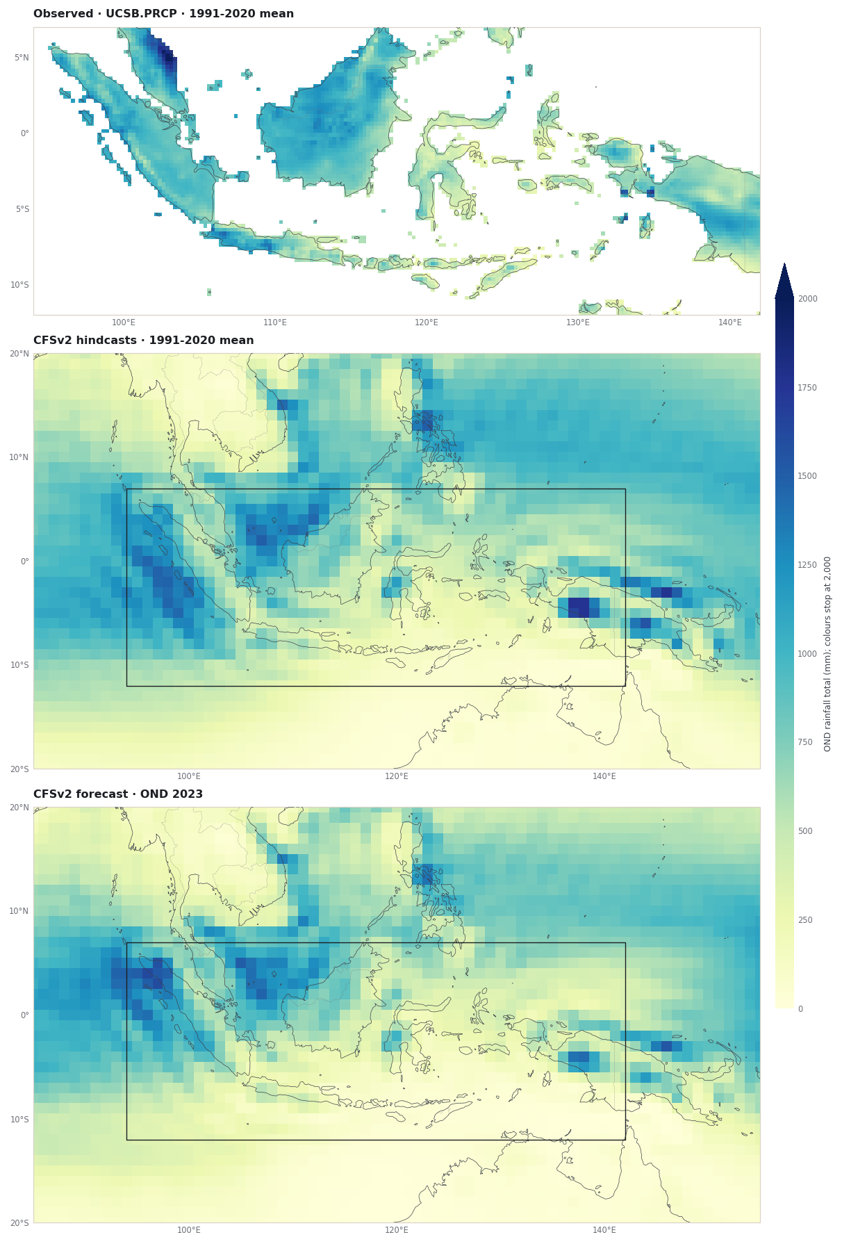
A map is the fastest check that nothing is shifted, flipped or empty. The panels show the 1991-2020 average of the observed OND totals, the same average of the CFSv2 hindcasts, and the 2023 forecast.
The observed field has values only over land; sea cells are the missing values counted in step 6. The black outline on the model panels is the predictand box. The model fields cover the whole predictor box, land and sea. All three panels share one colour scale, which stops at 2,000 mm; cells above it take the darkest colour.
What you have now
Observations, hindcasts and a forecast in the case folder, as .tsv and .nc.
A year-by-year availability check for the training period.
Evidence that these downloads did not use the IRI key.
Evidence that the values are seasonal totals in mm despite the mm/day label.
A measured difference between PyCPT’s CFSv2 totals and the Fit & diagnose inputs, explained exactly by how the three months are weighted.
The next chapter replaces the catalog observations with the local CHIRPS v3.0 file used by the case studies.
Saha, S., Moorthi, S., Wu, X., et al. (2014). The NCEP Climate Forecast System Version 2. Journal of Climate, 27(6), 2185-2208. https://doi.org/10.1175/JCLI-D-12-00823.1
Kirtman, B., Min, D., Infanti, J., et al. (2014). The North American Multimodel Ensemble: Phase-1 seasonal-to-interannual prediction; Phase-2 toward developing intraseasonal prediction. Bulletin of the American Meteorological Society, 95(4), 585-601. https://doi.org/10.1175/BAMS-D-12-00050.1
IRI Data Library. UCSB CHIRPS version 2.0. https://iridl.ldeo.columbia.edu/SOURCES/.UCSB/.CHIRPS/.v2p0/ Browsing Data Library pages requires signing in (checked 10 November 2026); PyCPT’s data requests in this tutorial succeeded without a key.
Funk, C., Peterson, P., Landsfeld, M., et al. (2015). The climate hazards infrared precipitation with stations: a new environmental record for monitoring extremes. Scientific Data, 2, 150066. https://doi.org/10.1038/sdata.2015.66