Issued 1 November 2023: the next six seasons

Three-month rainfall forecasts for Indonesia from one CFSv2 start, December-February to May-July, calibrated with CCA and PCR

A forecast centre issues an outlook on one date and looks several seasons ahead. This notebook does exactly that: it takes the CFSv2 run started on 1 November 2023 and makes a calibrated forecast for each of the next six seasons, from December-February to May-July. Lead 1 is the season starting one month after the issue date, lead 6 the one starting six months after it.

Because each lead is a different calendar season, a change in skill from one lead to the next mixes two things: forecasting further ahead, and some seasons being easier to forecast than others. Section 6 separates them by doing the opposite as well: one target, October-December 2023, forecast from six earlier starts.

NoteWhat you need to run this page

The full PyCPT environment with its CPT engine, internet access the first time (CFSv2 files from the IRI Data Library, no key needed), and the CHIRPS v3.0 dekadal archive described in step 2. Eighteen fits take several minutes; times are printed below.

1. One issue date, six targets

The lead is the number of whole months between the issue date and the first day of the target. PyCPT counts each target month from the start to its middle, so its own leads are half a month larger (seasons of three months span three PyCPT leads). Training uses the target years 1991-2020, as PyCPT’s target_first_year and target_final_year define them: for a target in January or later, the 1 November starts are those of the year before. The cell asks PyCPT for both.

from pathlib import Path
import datetime as dt
import json
import re
import sys
import time

import matplotlib.pyplot as plt
import numpy as np
import pandas as pd
import shapely
import xarray as xr
import cartopy.io.shapereader as shapereader
import cptdl as dl
import pycpt
from pycpt import notebook as pycpt_notebook

repo = next((p for p in (Path.cwd(), *Path.cwd().parents) if (p / "pycpt_tutorial").is_dir()), None)
if repo is None:
    raise FileNotFoundError("Run this notebook inside the tutorial repository or kit.")
sys.path.insert(0, str(repo))
from pycpt_tutorial.country_grid import aggregate_country_rainfall, training_complete_mask
from pycpt_tutorial.export import save_netcdf
from pycpt_tutorial import checks, figures
figures.use_style()

predictor_names = ["CFSv2.PRCP"]
predictand_name = "CHIRPS3.PRCP"
issue = dt.datetime(2023, 11, 1)
leads = [1, 2, 3, 4, 5, 6]                       # months from the issue date to the first day of the target
target_length = 3                          # months in each target
MONTHS = ["Jan", "Feb", "Mar", "Apr", "May", "Jun", "Jul", "Aug", "Sep", "Oct", "Nov", "Dec"]
targets = {lead: f"{MONTHS[(issue.month - 1 + lead) % 12]}-{MONTHS[(issue.month - 2 + lead + target_length) % 12]}"
           for lead in leads}
predictor_extent = {"west": 85, "east": 155, "south": -20, "north": 20}
predictand_extent = {"west": 94, "east": 142, "south": -12, "north": 7}
training_years = list(range(1991, 2021))          # target years
cpt_args = {
    "transform_predictand": None,
    "tailoring": None,
    "cca_modes": (2, 2),
    "x_eof_modes": (3, 3),
    "y_eof_modes": (3, 3),
    "validation": "crossvalidation",
    "drymask_threshold": None,
    "skillmask_threshold": None,
    "crossvalidation_window": 5,
    "synchronous_predictors": True,
}
force_download = False
case_root = Path.home() / "PyCPT" / "indonesia-issued-2023-11-seasons"

# Section 7: one target forecast from six earlier starts (the design of the earlier version of this case)
fixed_target = "Oct-Dec"
fixed_starts = {lead: dt.datetime(2023, 10 - lead, 1) for lead in leads}
fixed_root = Path.home() / "PyCPT" / "indonesia-ond-2023-leads"

rows = []
for lead, target in targets.items():
    low, high = dl.leads_from_target(issue, target)
    delta = pycpt_notebook.issue_year_delta(issue.month, target)
    rows.append({"lead (months)": lead, "target": target, "PyCPT lead": f"{low} to {high}",
                 "hindcast starts": f"1 Nov {training_years[0] + delta}-{training_years[-1] + delta}",
                 "2023 start": issue.strftime("%d %b %Y")})
pd.DataFrame(rows).set_index("lead (months)")
target PyCPT lead hindcast starts 2023 start
lead (months)
1 Dec-Feb 1.5 to 3.5 1 Nov 1990-2019 01 Nov 2023
2 Jan-Mar 2.5 to 4.5 1 Nov 1990-2019 01 Nov 2023
3 Feb-Apr 3.5 to 5.5 1 Nov 1990-2019 01 Nov 2023
4 Mar-May 4.5 to 6.5 1 Nov 1990-2019 01 Nov 2023
5 Apr-Jun 5.5 to 7.5 1 Nov 1990-2019 01 Nov 2023
6 May-Jul 6.5 to 8.5 1 Nov 1990-2019 01 Nov 2023

2. Observations from dekads

The predictand is CHIRPS v3.0 rainfall from the local dekadal archive (three accumulation periods per month: days 1-10, 11-20 and 21 to the end), the same archive family as chapter 3. Its metadata says exact zeros are kept. A target total is the sum of the dekads that tile it. The function below finds them from the stored time bounds and refuses to sum unless they run contiguously from the target’s first day to the day after its last.

chirps3_file = Path("/mnt/e/temp/chirps/dekad/wld_cli_chirps3_dekad_1981_2025.nc")
source = xr.open_dataset(chirps3_file)
print("Variable attributes:", {k: source.precip.attrs[k] for k in ("units", "cell_methods", "comment")})
bounds = pd.DatetimeIndex(source.time_bnds.values.ravel()).values.reshape(-1, 2)
dekad_first, dekad_end = pd.DatetimeIndex(bounds[:, 0]), pd.DatetimeIndex(bounds[:, 1])
print(f"Dekads in the archive: {len(dekad_first)}, {dekad_first[0]:%d %b %Y} to {dekad_end[-1]:%d %b %Y}")
box = predictand_extent
region = source.precip.sel(lon=slice(box["west"], box["east"]), lat=slice(box["south"], box["north"]))


def period_total(first, last):
    # Sum of the dekads covering first..last (inclusive days), checked against the stored bounds.
    end = pd.Timestamp(last) + pd.Timedelta(days=1)
    index = np.flatnonzero((dekad_first >= pd.Timestamp(first)) & (dekad_end <= end))
    assert len(index) > 0 and dekad_first[index[0]] == pd.Timestamp(first) and dekad_end[index[-1]] == end, (first, last)
    assert (dekad_first[index[1:]] == dekad_end[index[:-1]]).all(), (first, last)
    return region.isel(time=index).sum("time", skipna=False)
Variable attributes: {'units': 'mm', 'cell_methods': 'time: sum', 'comment': 'Exact zeros are preserved, for a zero-inflated distribution fit. NaN marks no data.'}
Dekads in the archive: 1620, 01 Jan 1981 to 01 Jan 2026

A consistency check against a separately stored product: the archive also has 3-month totals (the file chapter 3 used). December-February built from nine dekads should equal the stored total. The cell compares them for the first training season and for the 2023-24 season.

rolling = xr.open_dataset("/mnt/e/temp/chirps/rolling_dekad/wld_cli_chirps3_month3_bydekad_1981_2025.nc")
rolling_first = pd.DatetimeIndex(rolling.time_bnds.values[:, 0])
rolling_end = pd.DatetimeIndex(rolling.time_bnds.values[:, 1])
for year in [1990, 2023]:
    first, last = pd.Timestamp(year, 12, 1), pd.Timestamp(year + 1, 2, 1) + pd.offsets.MonthEnd(0)
    k = int(np.flatnonzero((rolling_first == first) & (rolling_end == last + pd.Timedelta(days=1)))[0])
    stored = rolling.precip.sel(lon=slice(box["west"], box["east"]), lat=slice(box["south"], box["north"])).isel(time=k).load()
    from_dekads = period_total(first, last).load()
    gap = abs(from_dekads - stored)
    print(f"DJF {year}-{(year + 1) % 100:02d} ({first:%d %b %Y} to {last:%d %b %Y}): largest difference {float(gap.max()):.4f} mm, "
          f"same missing pixels: {bool((from_dekads.isnull() == stored.isnull()).all())}")
DJF 1990-91 (01 Dec 1990 to 28 Feb 1991): largest difference 0.0002 mm, same missing pixels: True
DJF 2023-24 (01 Dec 2023 to 29 Feb 2024): largest difference 0.0005 mm, same missing pixels: True

The predictand keeps CHIRPS v3.0’s native 0.05° grid: every pixel whose centre lies inside Indonesia (Natural Earth 1:10m), with no averaging to coarser cells. A pixel enters the fits only if it has data in all 30 training years of every target used on this page (the six leads and the OND target of section 6), so every area mean covers the same pixels. Area means weight each pixel by the cosine of its latitude.

records = shapereader.Reader(shapereader.natural_earth("10m", "cultural", "admin_0_countries")).records()
indonesia = next(r.geometry for r in records if r.attributes["ADM0_A3"] == "IDN")
shapely.prepare(indonesia)
lon2d, lat2d = np.meshgrid(region.lon, region.lat)
country = xr.DataArray(shapely.contains_xy(indonesia, lon2d, lat2d), dims=("lat", "lon"),
                       coords={"lat": region.lat, "lon": region.lon})
print(f"Native pixels inside Indonesia: {int(country.sum()):,}")


def observed_cells(data):
    # Target totals at the native 0.05 degree pixels inside Indonesia, on the T, Ti, Tf axis of a PyCPT file.
    native = xr.concat([period_total(a, b) for a, b in zip(data["Ti"].values, data["Tf"].values)],
                       dim=pd.Index(data["T"].values, name="T")).load()
    zeros = int(((native == 0) & country).sum())
    pixels = native.where(country).rename({"lat": "Y", "lon": "X"})
    pixels = pixels.assign_coords(Y=np.round(pixels["Y"].values.astype(float), 3), X=np.round(pixels["X"].values.astype(float), 3))
    pixels = pixels.sortby("Y", ascending=False).astype("float32")
    return pixels.assign_coords(Ti=("T", data["Ti"].values), Tf=("T", data["Tf"].values)), zeros
Native pixels inside Indonesia: 61,192

3. One case folder per lead

Each lead is its own forecast question, so each gets its own case folder (chapter 7 explains why folders should not be shared between questions). The hindcasts are downloaded first, because their T, Ti and Tf say exactly which days each training target covers; the observations are then built for those days and saved as that folder’s local predictand file. The OND starts of section 6 are prepared the same way.

def prepare(name, args, folder):
    domain_dir = pycpt.setup(folder, predictor_extent)
    hindcasts = pycpt_notebook.download_hindcasts(predictor_names, domain_dir, force_download, args)[0]
    assert (pd.DatetimeIndex(hindcasts["T"].values).year == np.array(training_years)).all()
    Yl, zeros = observed_cells(hindcasts)
    return dict(name=name, args=args, domain_dir=domain_dir, folder=folder, Y_all=Yl, zeros=zeros,
                complete=training_complete_mask(Yl, training_years))


start = time.monotonic()
questions = {}
for lead, target in targets.items():
    args = dict(fdate=issue, target=target, target_first_year=training_years[0], target_final_year=training_years[-1],
                predictor_extent=predictor_extent, predictand_extent=predictand_extent)
    questions["issue", lead] = prepare(target, args, case_root / f"lead-{lead}")
for lead, fdate in fixed_starts.items():
    args = dict(fdate=fdate, target=fixed_target, target_first_year=training_years[0], target_final_year=training_years[-1],
                predictor_extent=predictor_extent, predictand_extent=predictand_extent)
    questions["fixed", lead] = prepare(fixed_target, args, fixed_root / f"lead-{lead}")
cells = xr.concat([q["complete"] for q in questions.values()], "q").all("q")
print(f"Hindcast axes and observations for {len(questions)} questions in {time.monotonic() - start:.0f} s")
print(f"Pixels with data in all 30 training years of every target: {int(cells.sum()):,} "
      f"(per target: {sorted({int(q['complete'].sum()) for q in questions.values()})})")
print("Indonesian native pixel-targets at exactly 0 mm, by lead:",
      {lead: questions["issue", lead]["zeros"] for lead in leads})
Input data will be saved in ~/PyCPT/indonesia-issued-2023-11-seasons/lead-1/85W-155E_to_-20S-20N/data
Figures will be saved in ~/PyCPT/indonesia-issued-2023-11-seasons/lead-1/85W-155E_to_-20S-20N/figures
Output will be saved in ~/PyCPT/indonesia-issued-2023-11-seasons/lead-1/85W-155E_to_-20S-20N/output
Reusing already-downloaded CFSv2.PRCP

Input data will be saved in ~/PyCPT/indonesia-issued-2023-11-seasons/lead-2/85W-155E_to_-20S-20N/data
Figures will be saved in ~/PyCPT/indonesia-issued-2023-11-seasons/lead-2/85W-155E_to_-20S-20N/figures
Output will be saved in ~/PyCPT/indonesia-issued-2023-11-seasons/lead-2/85W-155E_to_-20S-20N/output
Reusing already-downloaded CFSv2.PRCP

Input data will be saved in ~/PyCPT/indonesia-issued-2023-11-seasons/lead-3/85W-155E_to_-20S-20N/data
Figures will be saved in ~/PyCPT/indonesia-issued-2023-11-seasons/lead-3/85W-155E_to_-20S-20N/figures
Output will be saved in ~/PyCPT/indonesia-issued-2023-11-seasons/lead-3/85W-155E_to_-20S-20N/output
Reusing already-downloaded CFSv2.PRCP

Input data will be saved in ~/PyCPT/indonesia-issued-2023-11-seasons/lead-4/85W-155E_to_-20S-20N/data
Figures will be saved in ~/PyCPT/indonesia-issued-2023-11-seasons/lead-4/85W-155E_to_-20S-20N/figures
Output will be saved in ~/PyCPT/indonesia-issued-2023-11-seasons/lead-4/85W-155E_to_-20S-20N/output
Reusing already-downloaded CFSv2.PRCP

Input data will be saved in ~/PyCPT/indonesia-issued-2023-11-seasons/lead-5/85W-155E_to_-20S-20N/data
Figures will be saved in ~/PyCPT/indonesia-issued-2023-11-seasons/lead-5/85W-155E_to_-20S-20N/figures
Output will be saved in ~/PyCPT/indonesia-issued-2023-11-seasons/lead-5/85W-155E_to_-20S-20N/output
Reusing already-downloaded CFSv2.PRCP

Input data will be saved in ~/PyCPT/indonesia-issued-2023-11-seasons/lead-6/85W-155E_to_-20S-20N/data
Figures will be saved in ~/PyCPT/indonesia-issued-2023-11-seasons/lead-6/85W-155E_to_-20S-20N/figures
Output will be saved in ~/PyCPT/indonesia-issued-2023-11-seasons/lead-6/85W-155E_to_-20S-20N/output
Reusing already-downloaded CFSv2.PRCP

Input data will be saved in ~/PyCPT/indonesia-ond-2023-leads/lead-1/85W-155E_to_-20S-20N/data
Figures will be saved in ~/PyCPT/indonesia-ond-2023-leads/lead-1/85W-155E_to_-20S-20N/figures
Output will be saved in ~/PyCPT/indonesia-ond-2023-leads/lead-1/85W-155E_to_-20S-20N/output
Reusing already-downloaded CFSv2.PRCP

Input data will be saved in ~/PyCPT/indonesia-ond-2023-leads/lead-2/85W-155E_to_-20S-20N/data
Figures will be saved in ~/PyCPT/indonesia-ond-2023-leads/lead-2/85W-155E_to_-20S-20N/figures
Output will be saved in ~/PyCPT/indonesia-ond-2023-leads/lead-2/85W-155E_to_-20S-20N/output
Reusing already-downloaded CFSv2.PRCP

Input data will be saved in ~/PyCPT/indonesia-ond-2023-leads/lead-3/85W-155E_to_-20S-20N/data
Figures will be saved in ~/PyCPT/indonesia-ond-2023-leads/lead-3/85W-155E_to_-20S-20N/figures
Output will be saved in ~/PyCPT/indonesia-ond-2023-leads/lead-3/85W-155E_to_-20S-20N/output
Reusing already-downloaded CFSv2.PRCP

Input data will be saved in ~/PyCPT/indonesia-ond-2023-leads/lead-4/85W-155E_to_-20S-20N/data
Figures will be saved in ~/PyCPT/indonesia-ond-2023-leads/lead-4/85W-155E_to_-20S-20N/figures
Output will be saved in ~/PyCPT/indonesia-ond-2023-leads/lead-4/85W-155E_to_-20S-20N/output
Reusing already-downloaded CFSv2.PRCP

Input data will be saved in ~/PyCPT/indonesia-ond-2023-leads/lead-5/85W-155E_to_-20S-20N/data
Figures will be saved in ~/PyCPT/indonesia-ond-2023-leads/lead-5/85W-155E_to_-20S-20N/figures
Output will be saved in ~/PyCPT/indonesia-ond-2023-leads/lead-5/85W-155E_to_-20S-20N/output
Reusing already-downloaded CFSv2.PRCP

Input data will be saved in ~/PyCPT/indonesia-ond-2023-leads/lead-6/85W-155E_to_-20S-20N/data
Figures will be saved in ~/PyCPT/indonesia-ond-2023-leads/lead-6/85W-155E_to_-20S-20N/figures
Output will be saved in ~/PyCPT/indonesia-ond-2023-leads/lead-6/85W-155E_to_-20S-20N/output
Reusing already-downloaded CFSv2.PRCP

Hindcast axes and observations for 12 questions in 118 s
Pixels with data in all 30 training years of every target: 61,190 (per target: [61190])
Indonesian native pixel-targets at exactly 0 mm, by lead: {1: 0, 2: 0, 3: 0, 4: 0, 5: 0, 6: 1}
inputs, rows, warnings = {}, [], set()
for key, q in questions.items():
    Yl = q["Y_all"].where(cells).transpose("T", "Y", "X").rename("precipitation")
    Yl.attrs = {"units": "mm", "missing": -999.0,
                "long_name": f"CHIRPS v3.0 {q['name']} rainfall total, Indonesia land, native 0.05 degree"}
    local_file = q["folder"] / f"local-CHIRPS3-{q['name']}-1991-2020.nc"
    save_netcdf(Yl.to_dataset(), local_file, overwrite=True,
                metadata={"source_file": chirps3_file.name,
                          "aggregation": "sum of the dekads tiling each target; native 0.05 degree pixels whose centre lies inside Indonesia",
                          "boundary": "Natural Earth 1:10m admin_0_countries, ADM0_A3=IDN",
                          "training_years": "target years 1991-2020"})
    checks.remember_question(q["args"], q["domain_dir"])
    Yd, X, F = pycpt.download_data(predictand_name, local_file, predictor_names, q["args"], q["domain_dir"], force_download)
    same_axis = bool((X[0]["T"].values == Yl["T"].values).all() and (X[0]["Ti"].values == Yl["Ti"].values).all()
                     and (X[0]["Tf"].values == Yl["Tf"].values).all())
    table = checks.check_case(q["args"], predictand_name, Yd, X, F, predictor_names, q["domain_dir"])
    warnings |= {f"{r.check}: {r.detail}" for r in table.itertuples() if r.status == "warn"}
    inputs[key] = dict(q, Y=Yd, Yl=Yl, X=X, F=F)
    s0, f0 = pd.Timestamp(X[0]["S"].values[0]), pd.Timestamp(F[0]["S"].values[0])
    rows.append({"design": key[0], "lead": key[1], "target": q["name"],
                 "hindcast starts": f"{s0:%d %b} {s0.year}-{pd.Timestamp(X[0]['S'].values[-1]).year}",
                 "training targets": f"{pd.Timestamp(Yl['Ti'].values[0]):%d %b %Y} ... {pd.Timestamp(Yl['Tf'].values[-1]):%d %b %Y}",
                 "forecast start": f"{f0:%d %b %Y}",
                 "forecast target": f"{pd.Timestamp(F[0]['Ti'].values[0]):%d %b %Y} to {pd.Timestamp(F[0]['Tf'].values[0]):%d %b %Y}",
                 "same T, Ti, Tf as Y": same_axis, "preflight": checks.summary(table)})
print("Preflight warnings (all questions):", *sorted(warnings), sep="\n  ")
pd.DataFrame(rows).set_index(["design", "lead"])
Reusing already-downloaded CFSv2.PRCP_f2023

Using local observed predictand dataset
Reusing already-downloaded CFSv2.PRCP

Reusing already-downloaded CFSv2.PRCP_f2023

Using local observed predictand dataset
Reusing already-downloaded CFSv2.PRCP

Reusing already-downloaded CFSv2.PRCP_f2023

Using local observed predictand dataset
Reusing already-downloaded CFSv2.PRCP

Reusing already-downloaded CFSv2.PRCP_f2023

Using local observed predictand dataset
Reusing already-downloaded CFSv2.PRCP

Reusing already-downloaded CFSv2.PRCP_f2023

Using local observed predictand dataset
Reusing already-downloaded CFSv2.PRCP

Reusing already-downloaded CFSv2.PRCP_f2023

Using local observed predictand dataset
Reusing already-downloaded CFSv2.PRCP

Reusing already-downloaded CFSv2.PRCP_f2023

Using local observed predictand dataset
Reusing already-downloaded CFSv2.PRCP

Reusing already-downloaded CFSv2.PRCP_f2023

Using local observed predictand dataset
Reusing already-downloaded CFSv2.PRCP

Reusing already-downloaded CFSv2.PRCP_f2023

Using local observed predictand dataset
Reusing already-downloaded CFSv2.PRCP

Reusing already-downloaded CFSv2.PRCP_f2023

Using local observed predictand dataset
Reusing already-downloaded CFSv2.PRCP

Reusing already-downloaded CFSv2.PRCP_f2023

Using local observed predictand dataset
Reusing already-downloaded CFSv2.PRCP

Reusing already-downloaded CFSv2.PRCP_f2023

Using local observed predictand dataset
Reusing already-downloaded CFSv2.PRCP

Preflight warnings (all questions):
  CFSv2.PRCP: units label: units attribute is 'mm/day', a rate; the catalog requests examined in chapter 1 multiply by the season length, so confirm whether the values are rates or seasonal totals.
target hindcast starts training targets forecast start forecast target same T, Ti, Tf as Y preflight
design lead
issue 1 Dec-Feb 01 Nov 1990-2019 01 Dec 1990 ... 29 Feb 2020 01 Nov 2023 01 Dec 2023 to 29 Feb 2024 True {'ok': 10, 'warn': 1, 'fail': 0}
2 Jan-Mar 01 Nov 1990-2019 01 Jan 1991 ... 31 Mar 2020 01 Nov 2023 01 Jan 2024 to 31 Mar 2024 True {'ok': 10, 'warn': 1, 'fail': 0}
3 Feb-Apr 01 Nov 1990-2019 01 Feb 1991 ... 30 Apr 2020 01 Nov 2023 01 Feb 2024 to 30 Apr 2024 True {'ok': 10, 'warn': 1, 'fail': 0}
4 Mar-May 01 Nov 1990-2019 01 Mar 1991 ... 31 May 2020 01 Nov 2023 01 Mar 2024 to 31 May 2024 True {'ok': 10, 'warn': 1, 'fail': 0}
5 Apr-Jun 01 Nov 1990-2019 01 Apr 1991 ... 30 Jun 2020 01 Nov 2023 01 Apr 2024 to 30 Jun 2024 True {'ok': 10, 'warn': 1, 'fail': 0}
6 May-Jul 01 Nov 1990-2019 01 May 1991 ... 31 Jul 2020 01 Nov 2023 01 May 2024 to 31 Jul 2024 True {'ok': 10, 'warn': 1, 'fail': 0}
fixed 1 Oct-Dec 01 Sep 1991-2020 01 Oct 1991 ... 31 Dec 2020 01 Sep 2023 01 Oct 2023 to 31 Dec 2023 True {'ok': 10, 'warn': 1, 'fail': 0}
2 Oct-Dec 01 Aug 1991-2020 01 Oct 1991 ... 31 Dec 2020 01 Aug 2023 01 Oct 2023 to 31 Dec 2023 True {'ok': 10, 'warn': 1, 'fail': 0}
3 Oct-Dec 01 Jul 1991-2020 01 Oct 1991 ... 31 Dec 2020 01 Jul 2023 01 Oct 2023 to 31 Dec 2023 True {'ok': 10, 'warn': 1, 'fail': 0}
4 Oct-Dec 01 Jun 1991-2020 01 Oct 1991 ... 31 Dec 2020 01 Jun 2023 01 Oct 2023 to 31 Dec 2023 True {'ok': 10, 'warn': 1, 'fail': 0}
5 Oct-Dec 01 May 1991-2020 01 Oct 1991 ... 31 Dec 2020 01 May 2023 01 Oct 2023 to 31 Dec 2023 True {'ok': 10, 'warn': 1, 'fail': 0}
6 Oct-Dec 01 Apr 1991-2020 01 Oct 1991 ... 31 Dec 2020 01 Apr 2023 01 Oct 2023 to 31 Dec 2023 True {'ok': 10, 'warn': 1, 'fail': 0}

Units: the downloaded files say mm/day, but each request multiplies the daily mean by the number of days in the target (the /mul step in PyCPT’s request), so the values are totals in millimetres, as chapter 2 found. PyCPT’s month lengths give February 28.25 days in every year (monthlengths in cptdl/targetleadconv.py), while the observations have 28 or 29. Regression onto the observed totals absorbs a constant factor, and correlation ignores it. The cell reads the factor from each request and compares the hindcasts’ 1991-2020 mean with the observed mean.

weights = np.cos(np.deg2rad(cells["Y"])) * cells
rows = []
for lead in leads:
    d = inputs["issue", lead]
    url = dl.evaluate_url(dl.hindcasts[predictor_names[0]], **pycpt_notebook._preprocess_download_args(d["args"]))
    X = d["X"][0]
    X = X.where((X > -999) & (X["X"] >= box["west"]) & (X["X"] <= box["east"]) & (X["Y"] >= box["south"]) & (X["Y"] <= box["north"]))
    rows.append({"lead": lead, "target": d["name"], "units attribute": d["X"][0].attrs.get("units"),
                 "multiplied by (days)": float(re.search(r"/([\d.]+)/mul", url).group(1)),
                 "CFSv2 1991-2020 mean over the box (mm)": round(float(X.mean("T").weighted(np.cos(np.deg2rad(X["Y"]))).mean()), 1),
                 "observed 1991-2020 mean, Indonesian pixels (mm)": round(float(d["Yl"].mean("T").weighted(weights).mean()), 1)})
pd.DataFrame(rows).set_index("lead")
target units attribute multiplied by (days) CFSv2 1991-2020 mean over the box (mm) observed 1991-2020 mean, Indonesian pixels (mm)
lead
1 Dec-Feb mm/day 90.25 727.3 842.0
2 Jan-Mar mm/day 90.25 700.2 830.8
3 Feb-Apr mm/day 89.25 644.4 830.9
4 Mar-May mm/day 92.00 633.3 816.4
5 Apr-Jun mm/day 91.00 601.8 733.5
6 May-Jul mm/day 92.00 556.0 631.9

4. Twelve fits, and six more

CCA and PCR at each lead, with the settings fixed above, through PyCPT’s own evaluate_models; then CCA for the six starts of section 6. At 0.05° one fit takes several minutes, most of it spent writing and reading CPT’s files for 61,000 pixels, so the eighteen fits run side by side, each evaluate_models call in its own Python process with its own CPT workspace. As chapter 4 showed, the deterministic skill scores describe cross-validated hindcasts (window of 5), while the probabilistic ones are in-sample. Only the deterministic ones are used for skill below.

import multiprocessing
from concurrent.futures import ProcessPoolExecutor


def fit(job):
    # One PyCPT fit, in its own process (forked, so it shares the inputs above); CPT works in its own workspace.
    key, MOS = job
    d = inputs[key]
    start = time.monotonic()
    hcsts, fcsts, skill, pxs, pys = pycpt.evaluate_models(d["X"], MOS, d["Y"], d["F"], cpt_args, d["domain_dir"], predictor_names)
    return key + (MOS,), dict(fcsts=fcsts[0], skill=skill[0], seconds=time.monotonic() - start)


jobs = [(key, MOS) for key in inputs for MOS in (["CCA", "PCR"] if key[0] == "issue" else ["CCA"])]
start = time.monotonic()
with ProcessPoolExecutor(max_workers=len(jobs), mp_context=multiprocessing.get_context("fork")) as pool:
    results = dict(pool.map(fit, jobs))
print(f"{len(jobs)} fits in {(time.monotonic() - start) / 60:.0f} min wall time; minutes per fit:",
      {f"{k[0]}-{k[1]}-{k[2]}": round(r["seconds"] / 60, 1) for k, r in results.items()})
18 fits in 17 min wall time; minutes per fit: {'issue-1-CCA': 17.3, 'issue-1-PCR': 15.7, 'issue-2-CCA': 16.9, 'issue-2-PCR': 16.3, 'issue-3-CCA': 16.1, 'issue-3-PCR': 15.2, 'issue-4-CCA': 16.1, 'issue-4-PCR': 15.5, 'issue-5-CCA': 16.2, 'issue-5-PCR': 17.2, 'issue-6-CCA': 16.2, 'issue-6-PCR': 16.3, 'fixed-1-CCA': 16.3, 'fixed-2-CCA': 16.1, 'fixed-3-CCA': 17.2, 'fixed-4-CCA': 16.9, 'fixed-5-CCA': 16.2, 'fixed-6-CCA': 17.3}

5. Skill by lead

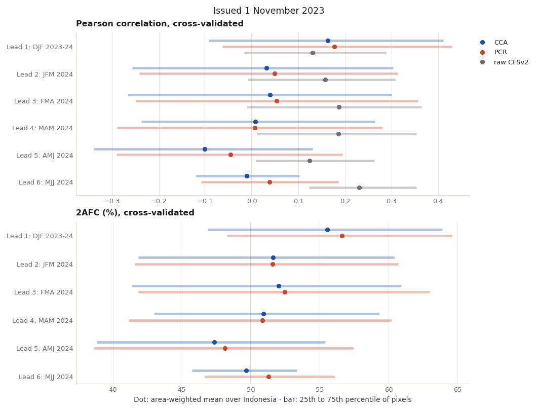
Each score is first computed at every pixel, then summarised over Indonesia as an area-weighted mean (weights: cosine of latitude). Three deterministic scores:

  • Pearson correlation of the cross-validated hindcasts with the observations, 1991-2020. Zero means no linear relationship.
  • 2AFC, the chance (in %) that the hindcasts rank two different years in the observed order. 50% is what a forecast without skill would get.
  • ROC area for below- and above-normal seasons. 0.5 is no skill.

The raw CFSv2 row is a baseline without calibration: the model’s own hindcasts, interpolated linearly from 1° to the pixel centres, correlated with the same observations. Correlation ignores the model’s bias, so this is a fair comparison for that one score.

Remember that each lead is also a different season: lead 1 is December -February, lead 6 is May-July.

grid_Y, grid_X = cells["Y"], cells["X"]


def on_grid(a):
    return a.where(a > -999).reindex(Y=grid_Y, X=grid_X, method="nearest", tolerance=1e-3)


def area_mean(field):
    return float(on_grid(field).where(cells).weighted(weights).mean(("Y", "X")))


def pearson(a, b):
    a, b = a - a.mean("T"), b - b.mean("T")
    return (a * b).sum("T") / np.sqrt((a * a).sum("T") * (b * b).sum("T"))


def raw_correlation(d):
    X = d["X"][0].where(d["X"][0] > -999).interp(Y=grid_Y, X=grid_X, method="linear")
    return pearson(X.reset_coords(drop=True), d["Yl"].reset_coords(drop=True)).where(cells)


label = {}
for lead in leads:
    F = inputs["issue", lead]["F"][0]
    a, b = pd.Timestamp(F["Ti"].values[0]), pd.Timestamp(F["Tf"].values[0])
    label[lead] = f"{a:%b %Y}" if target_length == 1 else (
        "".join(MONTHS[(a.month - 1 + k) % 12][0] for k in range(3)) + (f" {a.year}-{b.year % 100:02d}" if a.year != b.year else f" {a.year}"))
raw_pearson = {lead: raw_correlation(inputs["issue", lead]) for lead in leads}

rows = []
for lead in leads:
    for MOS in ["CCA", "PCR"]:
        s = results["issue", lead, MOS]["skill"]
        rows.append({"lead": lead, "target": label[lead], "method": MOS,
                     "Pearson": area_mean(s.pearson), "2AFC (%)": area_mean(s.two_alternative_forced_choice),
                     "ROC below normal": area_mean(s.roc_area_below_normal), "ROC above normal": area_mean(s.roc_area_above_normal),
                     "RMSE (mm)": area_mean(s.root_mean_squared_error)})
    rows.append({"lead": lead, "target": label[lead], "method": "raw CFSv2", "Pearson": area_mean(raw_pearson[lead])})
skill_by_lead = pd.DataFrame(rows).set_index(["lead", "method"]).sort_index()
skill_by_lead.round(3)
target Pearson 2AFC (%) ROC below normal ROC above normal RMSE (mm)
lead method
1 CCA DJF 2023-24 0.163 55.568 0.571 0.562 164.907
PCR DJF 2023-24 0.177 56.633 0.589 0.581 165.546
raw CFSv2 DJF 2023-24 0.131 NaN NaN NaN NaN
2 CCA JFM 2024 0.031 51.619 0.508 0.526 183.364
PCR JFM 2024 0.048 51.598 0.503 0.532 186.378
raw CFSv2 JFM 2024 0.157 NaN NaN NaN NaN
3 CCA FMA 2024 0.039 52.010 0.522 0.521 171.670
PCR FMA 2024 0.053 52.486 0.528 0.535 177.963
raw CFSv2 FMA 2024 0.187 NaN NaN NaN NaN
4 CCA MAM 2024 0.008 50.919 0.501 0.527 183.053
PCR MAM 2024 0.006 50.840 0.503 0.520 188.955
raw CFSv2 MAM 2024 0.186 NaN NaN NaN NaN
5 CCA AMJ 2024 -0.101 47.366 0.450 0.473 187.160
PCR AMJ 2024 -0.046 48.124 0.459 0.477 192.995
raw CFSv2 AMJ 2024 0.123 NaN NaN NaN NaN
6 CCA MJJ 2024 -0.011 49.659 0.467 0.521 199.904
PCR MJJ 2024 0.038 51.296 0.494 0.537 200.279
raw CFSv2 MJJ 2024 0.230 NaN NaN NaN NaN

The same numbers as a chart: one row per lead, the area-weighted mean as a dot, and the middle half of the pixels (25th to 75th percentile) as a bar, so the spread across Indonesia is visible alongside the average.

def quartiles(field):
    return np.nanpercentile(on_grid(field).where(cells).values, [25, 75])


series = {"CCA": figures.ACCENT, "PCR": figures.MARK, "raw CFSv2": figures.MUTED}
panels = [("Pearson", "pearson", "Pearson correlation, cross-validated", 0),
          ("2AFC (%)", "two_alternative_forced_choice", "2AFC (%), cross-validated", 50)]
fig, axes = plt.subplots(len(panels), 1, figsize=(figures.MAP_WIDTH, 7.2), layout="constrained")
for ax, (column, metric, title, reference) in zip(axes, panels):
    ax.axvline(reference, color=figures.LINE, linewidth=1)
    for k, (method, colour) in enumerate(series.items()):
        if method == "raw CFSv2" and metric != "pearson":
            continue
        offset = (k - 1) * 0.22
        for lead in leads:
            field = raw_pearson[lead] if method == "raw CFSv2" else results["issue", lead, method]["skill"][metric]
            low, high = quartiles(field)
            ax.plot([low, high], [lead + offset] * 2, color=colour, linewidth=3, alpha=.35, solid_capstyle="butt")
            ax.plot(skill_by_lead.loc[(lead, method), column], lead + offset, "o", color=colour, markersize=5,
                    label=method if lead == 1 else None)
    ax.set_yticks(leads, [f"Lead {lead}: {label[lead]}" for lead in leads])
    ax.invert_yaxis()
    ax.set_title(title)
    ax.grid(axis="y", visible=False)
axes[0].legend(loc="upper left", bbox_to_anchor=(1.0, 1.0))
axes[-1].set_xlabel("Dot: area-weighted mean over Indonesia · bar: 25th to 75th percentile of pixels")
fig.suptitle("Issued 1 November 2023")
assets = repo / "docs/assets/seasonal-leads-2023"
assets.mkdir(parents=True, exist_ok=True)
fig.savefig(assets / "skill-by-lead.png")
plt.show()

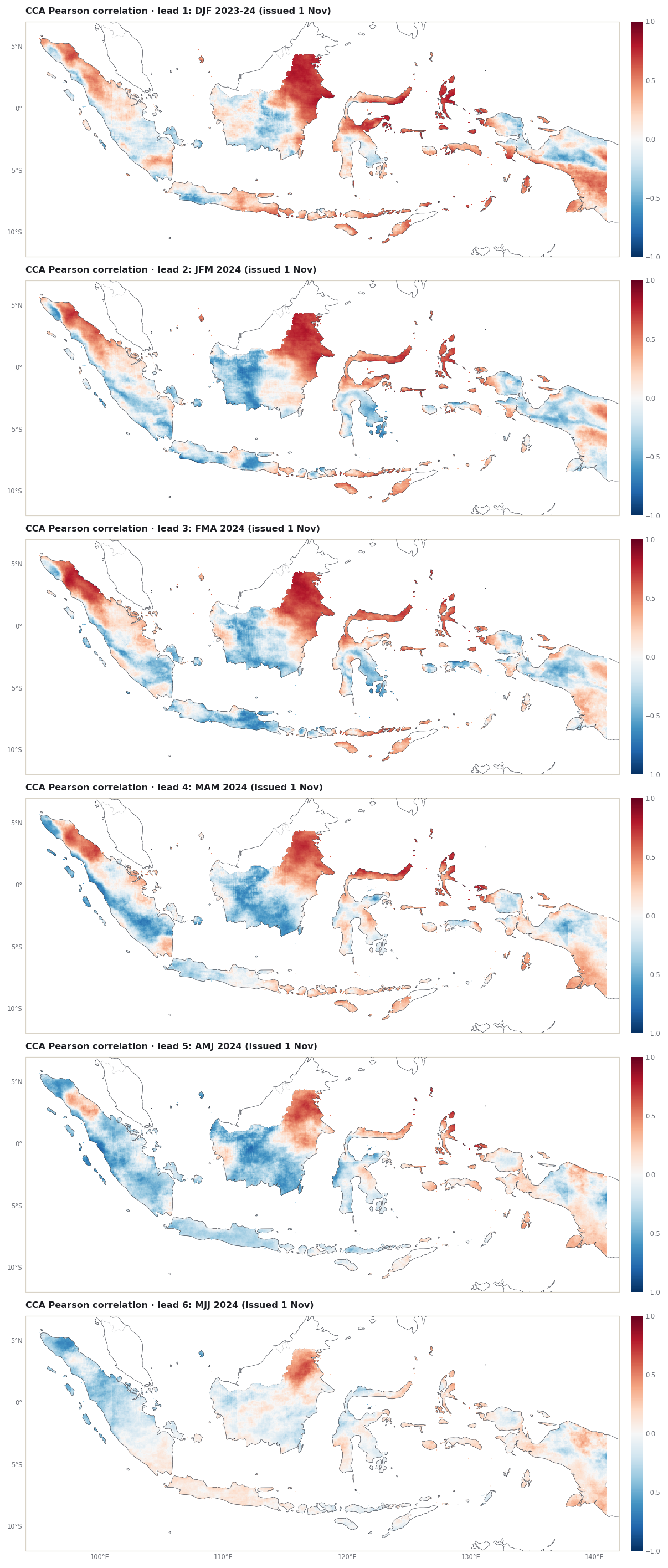
Where the skill sits matters as much as how much there is. The maps show the cross-validated CCA correlation at each lead, in one column from lead 1 (top) to lead 6 (bottom).

predictand_box = figures.extent_of(predictand_extent)
fig, grid = figures.stacked([figures.map_height(predictand_box)] * len(leads))
for row, lead in enumerate(leads):
    ax = figures.map_axes(fig, grid[row, 0], predictand_box, bottom_labels=row == len(leads) - 1)
    field = results["issue", lead, "CCA"]["skill"].pearson
    image = figures.draw_field(ax, field.where(field > -999), cmap="RdBu_r", vmin=-1, vmax=1)
    ax.set_title(f"CCA Pearson correlation · lead {lead}: {label[lead]} (issued 1 Nov)")
    figures.colorbar(fig, image, ax, "", ticks=[-1, -.5, 0, .5, 1])
fig.savefig(assets / "cca-pearson-by-lead.png")
plt.show()

6. Is it the lead or the season?

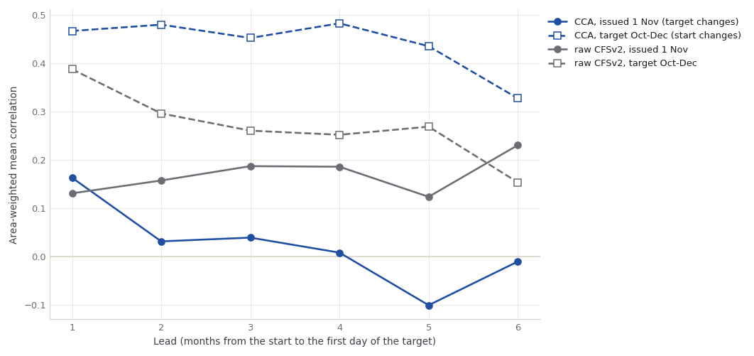
The same CCA settings, now for one target, October-December 2023, forecast from starts one to six months before it (1 September back to 1 April). Here the target is fixed and only the lead changes. Side by side with section 5, at each lead: if the two lines fall together, skill is mostly lost with lead time; if they part, the target season matters as much as how far ahead it is.

rows = []
for lead in leads:
    d = inputs["fixed", lead]
    rows.append({"lead": lead, "start": fixed_starts[lead].date().isoformat(), "target": d["name"],
                 "CCA Pearson": area_mean(results["fixed", lead, "CCA"]["skill"].pearson),
                 "raw CFSv2 Pearson": area_mean(raw_correlation(d)),
                 "CCA 2AFC (%)": area_mean(results["fixed", lead, "CCA"]["skill"].two_alternative_forced_choice)})
same_target = pd.DataFrame(rows).set_index("lead")
same_target["CCA Pearson, issued 1 Nov"] = [skill_by_lead.loc[(lead, "CCA"), "Pearson"] for lead in leads]
same_target["raw CFSv2 Pearson, issued 1 Nov"] = [skill_by_lead.loc[(lead, "raw CFSv2"), "Pearson"] for lead in leads]

fig, ax = plt.subplots(figsize=(figures.MAP_WIDTH, 4.4), layout="constrained")
ax.axhline(0, color=figures.LINE, linewidth=1)
for column, colour, style, name in [("CCA Pearson, issued 1 Nov", figures.ACCENT, "-o", "CCA, issued 1 Nov (target changes)"),
                                    ("CCA Pearson", figures.ACCENT, "--s", f"CCA, target {fixed_target} (start changes)"),
                                    ("raw CFSv2 Pearson, issued 1 Nov", figures.MUTED, "-o", "raw CFSv2, issued 1 Nov"),
                                    ("raw CFSv2 Pearson", figures.MUTED, "--s", f"raw CFSv2, target {fixed_target}")]:
    ax.plot(leads, same_target[column], style, color=colour, label=name, markerfacecolor="white" if "--" in style else colour)
ax.set_xticks(leads, [f"{lead}" for lead in leads])
ax.set_xlabel("Lead (months from the start to the first day of the target)")
ax.set_ylabel("Area-weighted mean correlation")
ax.legend(loc="upper left", bbox_to_anchor=(1.0, 1.0))
fig.savefig(assets / "same-target-vs-issue.png")
plt.show()
same_target.round(3)

start target CCA Pearson raw CFSv2 Pearson CCA 2AFC (%) CCA Pearson, issued 1 Nov raw CFSv2 Pearson, issued 1 Nov
lead
1 2023-09-01 Oct-Dec 0.467 0.388 66.583 0.163 0.131
2 2023-08-01 Oct-Dec 0.480 0.296 66.883 0.031 0.157
3 2023-07-01 Oct-Dec 0.452 0.260 66.372 0.039 0.187
4 2023-06-01 Oct-Dec 0.483 0.252 67.008 0.008 0.186
5 2023-05-01 Oct-Dec 0.435 0.269 65.859 -0.101 0.123
6 2023-04-01 Oct-Dec 0.327 0.153 61.803 -0.011 0.230

7. Seasons and months from the same start

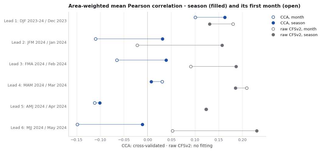
The monthly case used the same start (1 November 2023), model, observations, grid, settings and lead definition for single months, so the two can be set side by side: at each lead, the season and its first month. Its scores are read from the file that notebook saved.

monthly = pd.read_csv(repo / "docs/data/monthly-2023/skill-by-lead.csv").set_index(["lead", "method"])
rows = []
for lead in leads:
    for method in ["CCA", "PCR", "raw CFSv2"]:
        rows.append({"lead": lead, "method": method, "season": label[lead], "month": monthly.loc[(lead, method), "target"],
                     "Pearson, season": skill_by_lead.loc[(lead, method), "Pearson"],
                     "Pearson, month": monthly.loc[(lead, method), "Pearson"]})
comparison = pd.DataFrame(rows).set_index(["lead", "method"])
comparison["season minus month"] = comparison["Pearson, season"] - comparison["Pearson, month"]

fig, ax = plt.subplots(figsize=(figures.MAP_WIDTH, 4.4), layout="constrained")
ax.axvline(0, color=figures.LINE, linewidth=1)
for k, (method, colour) in enumerate([("CCA", figures.ACCENT), ("raw CFSv2", figures.MUTED)]):
    offset = (k - .5) * 0.3
    for lead in leads:
        a, b = comparison.loc[(lead, method), ["Pearson, month", "Pearson, season"]]
        ax.plot([a, b], [lead + offset] * 2, color=colour, linewidth=1.2, alpha=.5)
        ax.plot(a, lead + offset, "o", markerfacecolor="white", markeredgecolor=colour, markersize=6,
                label=f"{method}, month" if lead == 1 else None)
        ax.plot(b, lead + offset, "o", color=colour, markersize=6, label=f"{method}, season" if lead == 1 else None)
ax.set_yticks(leads, [f"Lead {lead}: {label[lead]} / {comparison.loc[(lead, 'CCA'), 'month']}" for lead in leads])
ax.invert_yaxis()
ax.grid(axis="y", visible=False)
ax.set_title("Area-weighted mean Pearson correlation · season (filled) and its first month (open)")
ax.set_xlabel("CCA: cross-validated · raw CFSv2: no fitting")
ax.legend(loc="upper left", bbox_to_anchor=(1.0, 1.0))
fig.savefig(assets / "seasonal-vs-monthly.png")
plt.show()
comparison.round(3)

season month Pearson, season Pearson, month season minus month
lead method
1 CCA DJF 2023-24 Dec 2023 0.163 0.101 0.062
PCR DJF 2023-24 Dec 2023 0.177 0.094 0.083
raw CFSv2 DJF 2023-24 Dec 2023 0.131 0.180 -0.050
2 CCA JFM 2024 Jan 2024 0.031 -0.110 0.141
PCR JFM 2024 Jan 2024 0.048 -0.092 0.140
raw CFSv2 JFM 2024 Jan 2024 0.157 -0.022 0.179
3 CCA FMA 2024 Feb 2024 0.039 -0.065 0.104
PCR FMA 2024 Feb 2024 0.053 -0.054 0.106
raw CFSv2 FMA 2024 Feb 2024 0.187 0.091 0.096
4 CCA MAM 2024 Mar 2024 0.008 0.031 -0.023
PCR MAM 2024 Mar 2024 0.006 0.009 -0.003
raw CFSv2 MAM 2024 Mar 2024 0.186 0.209 -0.023
5 CCA AMJ 2024 Apr 2024 -0.101 -0.112 0.011
PCR AMJ 2024 Apr 2024 -0.046 -0.093 0.047
raw CFSv2 AMJ 2024 Apr 2024 0.123 0.124 -0.001
6 CCA MJJ 2024 May 2024 -0.011 -0.148 0.137
PCR MJJ 2024 May 2024 0.038 -0.099 0.137
raw CFSv2 MJJ 2024 May 2024 0.230 0.052 0.178

8. The forecasts as issued, and what happened

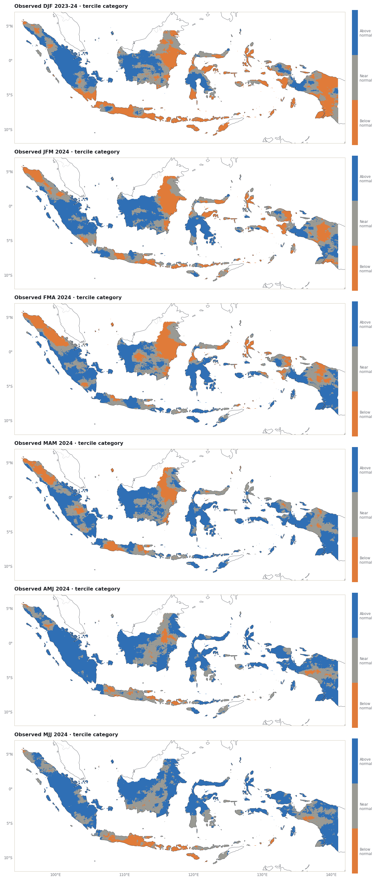
Each lead’s forecast is checked against its own target: December 2023-February 2024 to May-July 2024. The categories are defined as in chapter 5: at each pixel, below normal is under the 33rd percentile of that target’s 1991-2020 values and above normal over the 67th (NumPy’s hazen rule, which reproduces CPT’s own probabilities, as chapter 5 shows).

CATS = ["below normal", "near normal", "above normal"]
observed, reference_rows = {}, []
for lead in leads:
    d = inputs["issue", lead]
    obs, _ = observed_cells(d["F"][0])
    obs = obs.isel(T=0, drop=True).drop_vars(["Ti", "Tf"], errors="ignore").where(cells)
    Yl = d["Yl"]
    q = np.quantile(Yl.transpose("T", "Y", "X").values, [0.33, 0.67], axis=0, method="hazen")
    lower = xr.DataArray(q[0], coords={"Y": Yl["Y"], "X": Yl["X"]}, dims=("Y", "X")).where(cells)
    upper = lower.copy(data=q[1]).where(cells)
    category = xr.where(obs < lower, 0, xr.where(obs > upper, 2, 1)).where(cells & obs.notnull())
    mean = Yl.mean("T").where(cells)
    area = weights.where(category.notnull(), 0)
    shares = {name: float(area.where(category == k, 0).sum() / area.sum() * 100) for k, name in enumerate(CATS)}
    observed[lead] = dict(total=obs, mean=mean, category=category, shares=shares)
    reference_rows.append({"lead": lead, "target": label[lead],
                           "observed mean (mm)": float(obs.weighted(weights).mean()),
                           "1991-2020 mean (mm)": float(mean.weighted(weights).mean()),
                           **{f"observed {name} (% of area)": v for name, v in shares.items()},
                           "reference hit rate (%)": max(shares.values()),
                           "reference category": max(shares, key=shares.get)})
targets_2023 = pd.DataFrame(reference_rows).set_index("lead")
targets_2023.round(1)
target observed mean (mm) 1991-2020 mean (mm) observed below normal (% of area) observed near normal (% of area) observed above normal (% of area) reference hit rate (%) reference category
lead
1 DJF 2023-24 842.1 842.0 33.7 33.1 33.2 33.7 below normal
2 JFM 2024 871.2 830.8 23.6 34.6 41.8 41.8 above normal
3 FMA 2024 875.0 830.9 21.8 33.2 45.0 45.0 above normal
4 MAM 2024 920.0 816.4 12.4 32.5 55.1 55.1 above normal
5 AMJ 2024 881.2 733.5 4.6 28.6 66.8 66.8 above normal
6 MJJ 2024 734.3 631.9 6.7 31.9 61.4 61.4 above normal

Observed category at each lead’s target, in one column from lead 1 (top) to lead 6 (bottom).

def category_bar(fig, image, ax):
    # a colour bar with the three category names, so every map in a column has the same width
    bar = figures.colorbar(fig, image, ax, "", ticks=[0, 1, 2])
    bar.ax.set_yticklabels(["Below\nnormal", "Near\nnormal", "Above\nnormal"])
    return bar


fig, grid = figures.stacked([figures.map_height(predictand_box)] * len(leads))
for row, lead in enumerate(leads):
    ax = figures.map_axes(fig, grid[row, 0], predictand_box, bottom_labels=row == len(leads) - 1)
    category_bar(fig, figures.category_map(ax, observed[lead]["category"]), ax)
    ax.set_title(f"Observed {label[lead]} · tercile category")
fig.savefig(assets / "observed-by-lead.png")
plt.show()

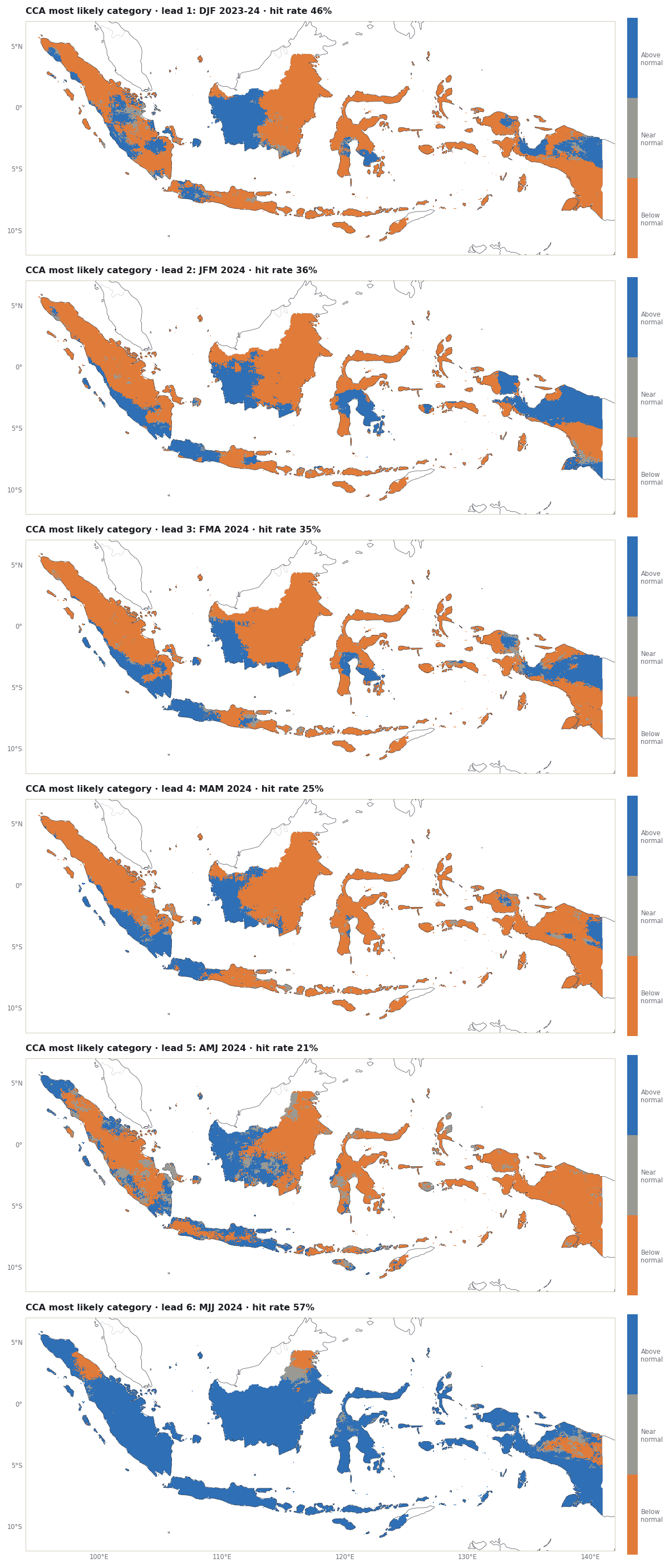
Now the forecasts. Each lead gives a probability for each category at each cell. Three ways to score them against what happened, each area-weighted over the pixels:

  • Hit rate: share of area where the most likely category was the one observed. Always forecasting one category would hit the area where that category happened; the reference hit rate above is the best such constant guess, chosen with hindsight.
  • RPSS: ranked probability skill score of this one target’s probabilities against climatological odds (33/34/33%). Above 0 means closer to what happened than climatology; it is one outcome, not a skill estimate.
  • RMSE: error of the deterministic forecast in mm.

The table also gives the share of the area where each category was the most likely one, to see whether a hit rate comes from placing categories well or from favouring the category that happened almost everywhere.

def rps(probability, category):
    cumulative = probability.cumsum("C") / 100
    outcome = xr.concat([(category <= k).astype(float) for k in range(3)], dim="C").assign_coords(C=probability["C"])
    return ((cumulative - outcome) ** 2).isel(C=slice(0, 2)).sum("C")


clim = xr.DataArray([33.0, 34.0, 33.0], dims="C")
forecast_rows, most_likely, deterministic = [], {}, {}
for lead in leads:
    o = observed[lead]
    valid = o["category"].notnull()
    for MOS in ["CCA", "PCR"]:
        f = results["issue", lead, MOS]["fcsts"]
        p = on_grid(f.probabilistic.isel(T=0))
        clim_p = clim.assign_coords(C=p["C"]).broadcast_like(p)
        m = p.fillna(-1).argmax("C").where(p.notnull().all("C") & valid)
        most_likely[lead, MOS] = (m, p.max("C"))
        w = weights.where(m.notnull(), 0)                       # pixels with both a forecast and an observation
        det = on_grid(f.deterministic.isel(T=0)).where(cells)
        deterministic[lead, MOS] = det
        forecast_rows.append({"lead": lead, "target": label[lead], "method": MOS,
                              "hit rate (%)": float(w.where(m == o["category"], 0).sum() / w.sum() * 100),
                              "RPSS": float(1 - rps(p, o["category"]).weighted(w).mean() / rps(clim_p, o["category"]).weighted(w).mean()),
                              "RMSE (mm)": float(np.sqrt(((det - o["total"]) ** 2).weighted(w).mean())),
                              "mean forecast (mm)": float(det.weighted(w).mean()),
                              "observed mean (mm)": float(o["total"].weighted(w).mean()),
                              **{f"area forecast {name} (%)": float(w.where(m == k, 0).sum() / w.sum() * 100)
                                 for k, name in enumerate(["below", "near", "above"])}})
forecast_2023 = pd.DataFrame(forecast_rows).set_index(["lead", "method"]).sort_index()
forecast_2023.round(2)
target hit rate (%) RPSS RMSE (mm) mean forecast (mm) observed mean (mm) area forecast below (%) area forecast near (%) area forecast above (%)
lead method
1 CCA DJF 2023-24 46.28 0.12 163.47 775.48 842.12 70.58 5.11 24.31
PCR DJF 2023-24 47.92 0.12 163.77 753.34 842.12 78.31 1.87 19.82
2 CCA JFM 2024 35.70 -0.01 170.42 791.71 871.21 65.59 1.87 32.54
PCR JFM 2024 40.17 0.03 164.92 800.97 871.21 56.38 4.19 39.44
3 CCA FMA 2024 34.76 -0.00 176.14 771.34 875.05 72.36 3.41 24.23
PCR FMA 2024 37.37 0.04 171.80 781.14 875.05 67.00 3.03 29.96
4 CCA MAM 2024 24.66 -0.16 225.32 759.88 920.00 79.32 3.19 17.49
PCR MAM 2024 28.32 -0.15 228.76 770.76 920.00 69.95 2.26 27.79
5 CCA AMJ 2024 21.15 -0.15 247.19 697.96 881.24 66.20 11.62 22.18
PCR AMJ 2024 38.75 -0.05 240.07 727.53 881.24 41.61 4.17 54.22
6 CCA MJJ 2024 56.91 0.16 157.58 717.06 734.31 6.65 4.45 88.90
PCR MJJ 2024 55.96 0.15 180.69 722.52 734.31 6.97 3.13 89.91

The CCA forecasts’ most likely category at each lead, in one column. Compare each map with the same lead in the observed column above.

fig, grid = figures.stacked([figures.map_height(predictand_box)] * len(leads))
for row, lead in enumerate(leads):
    ax = figures.map_axes(fig, grid[row, 0], predictand_box, bottom_labels=row == len(leads) - 1)
    category_bar(fig, figures.category_map(ax, most_likely[lead, "CCA"][0]), ax)
    hit = forecast_2023.loc[(lead, "CCA"), "hit rate (%)"]
    ax.set_title(f"CCA most likely category · lead {lead}: {label[lead]} · hit rate {hit:.0f}%")
fig.savefig(assets / "cca-category-by-lead.png")
plt.show()

9. Save the results

The story page quotes these tables and draws its interactive views from the JSON file written at the end.

data_dir = repo / "docs/data/seasonal-leads-2023"
data_dir.mkdir(parents=True, exist_ok=True)
skill_by_lead.round(4).to_csv(data_dir / "skill-by-lead.csv")
forecast_2023.round(4).to_csv(data_dir / "issued-2023-11-forecasts.csv")
targets_2023.round(4).to_csv(data_dir / "issued-2023-11-observed.csv")
same_target.round(4).to_csv(data_dir / "same-target-skill.csv")
if "comparison" in globals():
    comparison.round(4).to_csv(data_dir / "seasonal-vs-monthly.csv")
summary = {"issued": issue.date().isoformat(), "leads_months": leads,
           "targets": {lead: {"pycpt_target": targets[lead], "label": label[lead],
                               "first_day": str(inputs["issue", lead]["F"][0]["Ti"].values[0])[:10],
                               "last_day": str(inputs["issue", lead]["F"][0]["Tf"].values[0])[:10]} for lead in leads},
           "same_target": {"target": fixed_target, "starts": {lead: s.date().isoformat() for lead, s in fixed_starts.items()}},
           "training_target_years": [training_years[0], training_years[-1]], "pixels": int(cells.sum()), "grid": "native 0.05 degree",
           "settings": {k: str(v) for k, v in cpt_args.items()},
           "fit_seconds": {f"{k[0]}-{k[1]}-{k[2]}": round(r["seconds"], 1) for k, r in results.items()}}
(data_dir / "summary.json").write_text(json.dumps(summary, indent=2) + "\n")
maps = xr.Dataset()
for lead in leads:
    maps[f"observed_lead{lead}"] = observed[lead]["total"].reset_coords(drop=True)
    maps[f"observed_category_lead{lead}"] = observed[lead]["category"].reset_coords(drop=True)
    for MOS in ["CCA", "PCR"]:
        maps[f"{MOS.lower()}_pearson_lead{lead}"] = on_grid(results["issue", lead, MOS]["skill"].pearson).reset_coords(drop=True)
        maps[f"{MOS.lower()}_forecast_lead{lead}"] = deterministic[lead, MOS].reset_coords(drop=True)
        maps[f"{MOS.lower()}_most_likely_lead{lead}"] = most_likely[lead, MOS][0].reset_coords(drop=True)
save_netcdf(maps, data_dir / "seasonal-leads-2023-maps.nc", overwrite=True,
            metadata={"note": "CFSv2 started 1 November 2023, leads 1-6 months (DJF 2023-24 to MJJ 2024), CCA and PCR; categories 0 below, 1 near, 2 above normal"})
for f in sorted(data_dir.iterdir()) + sorted(assets.iterdir()):
    print(f"{f.relative_to(repo)}  ({f.stat().st_size / 1000:.0f} kB)")
docs/data/seasonal-leads-2023/issued-2023-11-forecasts.csv  (1 kB)
docs/data/seasonal-leads-2023/issued-2023-11-observed.csv  (1 kB)
docs/data/seasonal-leads-2023/same-target-skill.csv  (0 kB)
docs/data/seasonal-leads-2023/seasonal-leads-2023-maps.nc  (13441 kB)
docs/data/seasonal-leads-2023/seasonal-vs-monthly.csv  (1 kB)
docs/data/seasonal-leads-2023/skill-by-lead.csv  (1 kB)
docs/data/seasonal-leads-2023/summary.json  (2 kB)
docs/assets/seasonal-leads-2023/cca-category-by-lead.png  (1224 kB)
docs/assets/seasonal-leads-2023/cca-pearson-by-lead.png  (1985 kB)
docs/assets/seasonal-leads-2023/interactive-data.json  (1529 kB)
docs/assets/seasonal-leads-2023/observed-by-lead.png  (1209 kB)
docs/assets/seasonal-leads-2023/same-target-vs-issue.png  (104 kB)
docs/assets/seasonal-leads-2023/seasonal-vs-monthly.png  (88 kB)
docs/assets/seasonal-leads-2023/skill-by-lead.png  (111 kB)

The story page’s interactive maps and charts read a small manifest and, at 0.05°, one gzip-compressed binary file per map, loaded only when a view needs it: integers at a stated scale, stored only at the Indonesian pixels in the order of a shared pixel list.

import gzip


def records(frame):
    return [{k: (None if isinstance(v, float) and not np.isfinite(v) else v) for k, v in row.items()}
            for row in frame.to_dict(orient="records")]


field_dir = assets / "fields"
field_dir.mkdir(exist_ok=True)
for old in list(field_dir.glob("*")) + [assets / "interactive-data.json"]:
    old.unlink(missing_ok=True)
grid_mask = cells.transpose("Y", "X")
flat = np.flatnonzero(grid_mask.values.ravel())                    # row 0 = northernmost pixel row
n = len(flat)


def at_pixels(a):
    return np.asarray(on_grid(a).transpose("Y", "X").values, dtype="float64").ravel()[flat]


def encode(values, kind, scale):
    v = np.round(values * scale)
    if kind == "i16":
        return np.where(np.isfinite(v), np.clip(v, -32767, 32767), -32768).astype("<i2").tobytes()
    if kind == "u16":
        return np.where(np.isfinite(v), np.clip(v, 0, 65534), 65535).astype("<u2").tobytes()
    return np.where(np.isfinite(v), np.clip(v, 0, 254), 255).astype("u1").tobytes()


def write(name, parts):
    (field_dir / f"{name}.bin.gz").write_bytes(gzip.compress(b"".join(encode(*q) for q in parts), 9, mtime=0))


(assets / "pixels.bin").write_bytes(flat.astype("<i4").tobytes())
lead_key = {lead: f"lead{lead}" for lead in leads}
target_info, issue_targets = [], []
for lead in leads:
    F0 = inputs["issue", lead]["F"][0]
    first, last = pd.Timestamp(F0["Ti"].values[0]), pd.Timestamp(F0["Tf"].values[0])
    days = (last - first).days + 1
    target_info.append({"lead": lead, "label": label[lead], "pycpt": targets[lead], "start": f"{first:%Y-%m-%d}",
                        "end": f"{last + pd.Timedelta(days=1):%Y-%m-%d}"})
    issue_targets.append({"lead": lead_key[lead], "start": f"{first:%Y-%m-%d}", "days": int(days)})
    write(f"obs-{days}-{first:%Y-%m-%d}", [(at_pixels(observed[lead]["total"]), "u16", 10), (at_pixels(observed[lead]["mean"]), "u16", 10),
                                              (at_pixels(observed[lead]["category"]), "u8", 1)])
    for m in ["CCA", "PCR"]:
        write(f"skill-{m}-pearson-{lead_key[lead]}", [(at_pixels(results["issue", lead, m]["skill"].pearson), "i16", 1000)])
        write(f"skill-{m}-twoafc-{lead_key[lead]}", [(at_pixels(results["issue", lead, m]["skill"].two_alternative_forced_choice), "i16", 10)])
        write(f"fc-{lead_key[lead]}-{m}-{first:%Y-%m-%d}", [(at_pixels(deterministic[lead, m]), "u16", 10),
                                                                (at_pixels(most_likely[lead, m][0]), "u8", 1),
                                                                (at_pixels(most_likely[lead, m][1].where(cells)), "u8", 1)])
    write(f"skill-raw-pearson-{lead_key[lead]}", [(at_pixels(raw_pearson[lead]), "i16", 1000)])

values = np.concatenate([observed[lead]["total"].values.ravel() for lead in leads] + [deterministic[k].values.ravel() for k in deterministic])
top = float(np.ceil(np.nanpercentile(values, 99) / 100) * 100)
manifest = {
    "grid": {"west": round(float(grid_mask.X.min()) - .025, 3), "north": round(float(grid_mask.Y.max()) + .025, 3), "step": 0.05,
             "nx": int(grid_mask.sizes["X"]), "ny": int(grid_mask.sizes["Y"]), "pixels": n},
    "kind": "season", "issue": {"date": issue.date().isoformat(), "label": "1 Nov 2023"},
    "issues": [{"issued": issue.date().isoformat(), "label": "1 Nov 2023", "targets": issue_targets}],
    "leads": leads, "leadKeys": [lead_key[lead] for lead in leads], "methods": ["CCA", "PCR"], "rawName": "raw CFSv2", "unit": "mm",
    "training": "1991-2020", "sample": "the 30 training years, 1991-2020", "cellText": f"Indonesia's {n:,} pixels at 0.05°",
    "leadNames": [f"Lead {lead} · {label[lead]}" for lead in leads],
    "targets": target_info,
    "layout": {"skill": [["value", "i16"]], "obs": [["total", "u16", 10], ["mean", "u16", 10], ["category", "u8", 1]],
               "fc": [["total", "u16", 10], ["category", "u8", 1], ["probability", "u8", 1]]},
    "scales": {"pearson": 1000, "twoafc": 10},
    "rainMax": {str(t["days"]): top for t in issue_targets}, "rainLegend": "mm in the season",
    "mapsHint": "Lead 1 at the top. Each map is a different target; hover a pixel for the forecast, the observation and that target's 1991-2020 mean.",
    "skillTable": records(skill_by_lead.reset_index().round(4)),
    "scores2023": records(forecast_2023.reset_index().round(3)),
    "references": records(targets_2023.reset_index().round(3)),
    "sameTarget": {"target": "October-December 2023", "rows": records(same_target.reset_index().round(4))},
}
if "comparison" in globals():
    manifest["comparison"] = records(comparison.reset_index().round(4))
(assets / "manifest.json").write_text(json.dumps(manifest, separators=(",", ":"), allow_nan=False) + "\n")
sizes = sorted(q.stat().st_size for q in field_dir.iterdir())
print(f"{n:,} pixels; {len(sizes)} field files, {sum(sizes) / 1e6:.1f} MB in total (largest {sizes[-1] / 1e3:.0f} kB); "
      f"colour scale up to {top:.0f} mm")
61,190 pixels; 48 field files, 5.5 MB in total (largest 226 kB); colour scale up to 1600 mm

References

  1. IRI. PyCPT 2.10.4 source: pycpt/src/pycpt/notebook.py (setup, download_data, summarize_available_years, evaluate_models and the plotting functions). Tag pycpt-2.10.4, commit 084bb5c. https://github.com/iri-pycpt/pycpt/blob/084bb5c380c200b5f65f11ba224a965547b91da1/pycpt/src/pycpt/notebook.py
  2. IRI. PyCPT 2.10.4 source: cptdl (data catalog, leads_from_target, evaluate_url, download, simple_download). Tag pycpt-2.10.4, commit 084bb5c. https://github.com/iri-pycpt/pycpt/tree/084bb5c380c200b5f65f11ba224a965547b91da1/pycpt/src/cptdl
  3. IRI. CPT 17.8.3 source code archive. Columbia University Academic Commons. https://doi.org/10.7916/fdp6-v391
  4. CPT+. Forecast Probabilities (CPT help). https://cptplus.org/Help/Tools_Forecast_Probs.html Same page name as on the former cpthelp.iri.columbia.edu, which did not resolve when checked on 10 November 2026.
  5. IRI Data Library. NMME NCEP-CFSv2 hindcasts, PENTAD_SAMPLES_FULL, precipitation. https://iridl.ldeo.columbia.edu/SOURCES/.Models/.NMME/.NCEP-CFSv2/.HINDCAST/.PENTAD_SAMPLES_FULL/.prec/ Browsing Data Library pages requires signing in (checked 10 November 2026); PyCPT’s data requests in this tutorial succeeded without a key.
  6. Saha, S., Moorthi, S., Wu, X., et al. (2014). The NCEP Climate Forecast System Version 2. Journal of Climate, 27(6), 2185-2208. https://doi.org/10.1175/JCLI-D-12-00823.1
  7. Climate Hazards Center, UC Santa Barbara. CHIRPS: Rainfall Estimates from Rain Gauge and Satellite Observations (CHIRPS version 3.0 page). https://www.chc.ucsb.edu/data/chirps3
  8. Funk, C., Peterson, P., Landsfeld, M., et al. (2014). A quasi-global precipitation time series for drought monitoring. U.S. Geological Survey Data Series 832. https://doi.org/10.3133/ds832
  9. Natural Earth. Admin 0: Countries, 1:10m cultural vectors. https://www.naturalearthdata.com/downloads/10m-cultural-vectors/10m-admin-0-countries/
  10. Shapely. shapely.contains_xy. https://shapely.readthedocs.io/en/stable/reference/shapely.contains_xy.html
  11. NumPy. numpy.quantile (NumPy manual). https://numpy.org/doc/stable/reference/generated/numpy.quantile.html
  12. Mason, S. J., and Weigel, A. P. (2009). A generic forecast verification framework for administrative purposes. Monthly Weather Review, 137(1), 331-349. https://doi.org/10.1175/2008MWR2553.1
  13. Epstein, E. S. (1969). A scoring system for probability forecasts of ranked categories. Journal of Applied Meteorology, 8(6), 985-987. https://doi.org/10.1175/1520-0450(1969)008%3C0985:ASSFPF%3E2.0.CO;2
  14. Barnston, A. G., and van den Dool, H. M. (1993). A degeneracy in cross-validated skill in regression-based forecasts. Journal of Climate, 6(5), 963-977. https://doi.org/10.1175/1520-0442(1993)006%3C0963:ADICVS%3E2.0.CO;2
  15. SciTools. Cartopy (documentation). https://scitools.org.uk/cartopy/docs/latest/
Back to top