Choose ensemble members by a stated rule, calibrate each, and average them with construct_mme
So far every chapter used one model, CFSv2. PyCPT can calibrate several models and combine them into a multi-model ensemble (MME). This chapter does that in four steps: decide which models qualify, calibrate each with the same CCA settings, combine them with construct_mme, and measure what the ensemble changes compared with its members.
NoteWhat you need to run this page
The full PyCPT environment, the case folder from chapters 1 to 3, and internet access the first time, to download six more models from the IRI Data Library. Calibrating seven models takes several minutes; the time is printed below.
1. Which models qualify?
A model can join this ensemble only if the Data Library has its hindcasts for every September start from 1991 to 2020 and its September 2023 forecast. The rule was fixed before any skill was computed, so the ensemble is not chosen to look good.
Ten candidate catalog models were downloaded with download_data for exactly this question, and the result was recorded by this tutorial’s availability check. The cell reads that record.
from pathlib import Pathimport datetime as dtimport inspectimport jsonimport sysimport timeimport matplotlib.pyplot as pltimport numpy as npimport pandas as pdimport xarray as xrimport pycptfrom pycpt import notebook as pycpt_notebookrepo =next((p for p in (Path.cwd(), *Path.cwd().parents) if (p /"pycpt_tutorial").is_dir()), None)sys.path.insert(0, str(repo))from pycpt_tutorial import figuresfigures.use_style()records = json.loads((repo /"docs/data/learn/mme-availability.json").read_text())table = pd.DataFrame([{"model": r["model"],"training years missing": ", ".join(map(str, r["missing_training_years"])) or"none","2023 forecast": "yes"if r["forecast_present"] else"no","qualifies": "yes"if (not r["missing_training_years"] and r["forecast_present"]) else"no",} for r in records]).sort_values(["qualifies", "model"], ascending=[False, True]).set_index("model")table
training years missing
2023 forecast
qualifies
model
CCSM4.PRCP
none
yes
yes
CESM1.PRCP
none
yes
yes
CanSIPSIC3.PRCP
none
yes
yes
GEOSS2S.PRCP
none
yes
yes
SEAS51c.PRCP
none
yes
yes
SPEAR.PRCP
none
yes
yes
CanSIPSIC4.PRCP
none
no
no
GCFS2p1.PRCP
1991, 1992, 2020
yes
no
METEOFRANCE9.PRCP
1991, 1992
no
no
SPSv3p5.PRCP
1991, 1992, 2017, 2018, 2019, 2020
yes
no
Six candidates qualify. With CFSv2 from the earlier chapters, the ensemble has seven members. The table shows why the other four are left out: three of the Copernicus (C3S) models lack some training years, and two models have no September 2023 forecast in the catalog (one of them lacks both).
Input data will be saved in ~/PyCPT/indonesia-ond-2023-sep-init/85W-155E_to_-20S-20N/data
Figures will be saved in ~/PyCPT/indonesia-ond-2023-sep-init/85W-155E_to_-20S-20N/figures
Output will be saved in ~/PyCPT/indonesia-ond-2023-sep-init/85W-155E_to_-20S-20N/output
Ensemble: CFSv2.PRCP, CCSM4.PRCP, CESM1.PRCP, CanSIPSIC3.PRCP, GEOSS2S.PRCP, SEAS51c.PRCP, SPEAR.PRCP
2. Load the data and check the years
The availability check already downloaded these files into this case folder for the same question, so force_download=False reuses them; chapter 1 explains why that is safe only when the folder and question match. summarize_available_years confirms the training years for every member.
Y, hindcast_data, forecast_data = pycpt.download_data( predictand_name, local_predictand_file, predictor_names, download_args, domain_dir, force_download)pycpt.summarize_available_years(predictor_names, predictand_name, download_args, Y, hindcast_data, forecast_data)
Observations were retrieved for all years of the training period.
Hindcasts were retrieved for all years of the training period.
CHIRPS3.PRCP
CFSv2.PRCP
CCSM4.PRCP
CESM1.PRCP
CanSIPSIC3.PRCP
GEOSS2S.PRCP
SEAS51c.PRCP
SPEAR.PRCP
1991
ok
ok
ok
ok
ok
ok
ok
ok
1992
ok
ok
ok
ok
ok
ok
ok
ok
1993
ok
ok
ok
ok
ok
ok
ok
ok
1994
ok
ok
ok
ok
ok
ok
ok
ok
1995
ok
ok
ok
ok
ok
ok
ok
ok
1996
ok
ok
ok
ok
ok
ok
ok
ok
1997
ok
ok
ok
ok
ok
ok
ok
ok
1998
ok
ok
ok
ok
ok
ok
ok
ok
1999
ok
ok
ok
ok
ok
ok
ok
ok
2000
ok
ok
ok
ok
ok
ok
ok
ok
2001
ok
ok
ok
ok
ok
ok
ok
ok
2002
ok
ok
ok
ok
ok
ok
ok
ok
2003
ok
ok
ok
ok
ok
ok
ok
ok
2004
ok
ok
ok
ok
ok
ok
ok
ok
2005
ok
ok
ok
ok
ok
ok
ok
ok
2006
ok
ok
ok
ok
ok
ok
ok
ok
2007
ok
ok
ok
ok
ok
ok
ok
ok
2008
ok
ok
ok
ok
ok
ok
ok
ok
2009
ok
ok
ok
ok
ok
ok
ok
ok
2010
ok
ok
ok
ok
ok
ok
ok
ok
2011
ok
ok
ok
ok
ok
ok
ok
ok
2012
ok
ok
ok
ok
ok
ok
ok
ok
2013
ok
ok
ok
ok
ok
ok
ok
ok
2014
ok
ok
ok
ok
ok
ok
ok
ok
2015
ok
ok
ok
ok
ok
ok
ok
ok
2016
ok
ok
ok
ok
ok
ok
ok
ok
2017
ok
ok
ok
ok
ok
ok
ok
ok
2018
ok
ok
ok
ok
ok
ok
ok
ok
2019
ok
ok
ok
ok
ok
ok
ok
ok
2020
ok
ok
ok
ok
ok
ok
ok
ok
Forecast data
All forecasts were retrieved.
CFSv2.PRCP
CCSM4.PRCP
CESM1.PRCP
CanSIPSIC3.PRCP
GEOSS2S.PRCP
SEAS51c.PRCP
SPEAR.PRCP
2023
ok
ok
ok
ok
ok
ok
ok
3. Calibrate every member the same way
evaluate_models takes the whole list and fits CCA to each model in turn, with the settings of chapter 4. Each member is calibrated against the same CHIRPS v3.0 observations, so every member’s output is on the same 0.25° grid and in the same units, which is what makes averaging them possible.
Read it before using it. In PyCPT 2.10.4, construct_mme calls construct_mme_new and then evaluate_mme. The key lines of construct_mme_new:
source = inspect.getsource(pycpt_notebook.construct_mme_new).splitlines()for number, line inenumerate(source, start=1):ifany(word in line for word in ["fillna", ".mean('model')", "climo_prob =", "climo_var =", "climo_mu ="]):print(f"{number:4d} | {line}")
So the ensemble is an equal-weight average of the calibrated members, taken separately for the deterministic forecast, the prediction-error variance and the three category probabilities. A member with a missing value contributes climatology instead: its training mean, its hindcast variance or 33/34/33%. The ensemble probabilities are therefore averages of the members’ probabilities; they are not recomputed from the averaged forecast.
evaluate_mme then scores the averaged hindcasts. The deterministic hindcasts are averages of cross-validated hindcasts, so their scores are cross-validated. The probabilistic hindcasts are averages of the members’ in-sample probabilities (chapter 4, step 2), so the probabilistic scores inherit that optimism.
mme_det, mme_prob, mme_pev, mme_skill = pycpt.construct_mme( fcsts, hcsts, Y, ensemble, predictor_names, cpt_args, domain_dir)cells = Y.notnull().all("T")member_det = xr.concat([f.deterministic for f in fcsts], dim="model").mean("model")member_prob = xr.concat([f.probabilistic for f in fcsts], dim="model").mean("model")print("Ensemble forecast minus mean of members, largest difference:",float(abs(mme_det - member_det).where(cells).max()), "mm")print("Ensemble probabilities minus mean of members, largest difference:",float(abs(mme_prob - member_prob).where(cells).max()), "percentage points")print("Files written:", sorted(p.name for p in (domain_dir /"output").glob("MME_*")))
Ensemble forecast minus mean of members, largest difference: 0.0 mm
Ensemble probabilities minus mean of members, largest difference: 0.0 percentage points
Files written: ['MME_deterministic_forecast_2023.nc', 'MME_deterministic_hindcasts.nc', 'MME_forecast_prediction_error_variance_2023.nc', 'MME_hindcast_prediction_error_variance.nc', 'MME_probabilistic_forecast_2023.nc', 'MME_probabilistic_hindcasts.nc', 'MME_skill_scores.nc']
5. Did combining help? Cross-validated skill
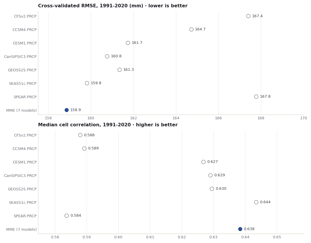
The fair comparison uses the cross-validated deterministic hindcasts, 1991-2020, over the 3,240 Indonesian cells. Two summaries per forecast: the error (RMSE, area-weighted, pooled over the 30 seasons) and the median of the cell-by-cell Pearson correlations that CPT reports.
Read the numbers above before reading this paragraph. In this case the ensemble has the lowest cross-validated RMSE of all eight forecasts, but not the highest median correlation, and the differences between the best members and the ensemble are small. Averaging reduces the error without making the ensemble better than every member on every measure.
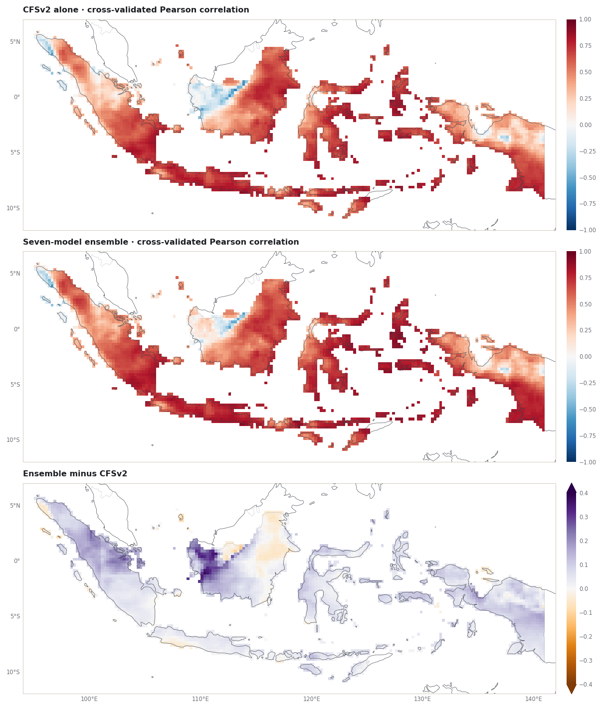
The dots are drawn on a scale that spans only the range of the eight values, so small differences look large; read the printed numbers. The maps show where the correlation changed, comparing the ensemble with CFSv2. In the third map, purple means the ensemble’s correlation is higher.
Cells where the ensemble correlation is higher than CFSv2's: 87.8%
6. The ensemble forecast for OND 2023
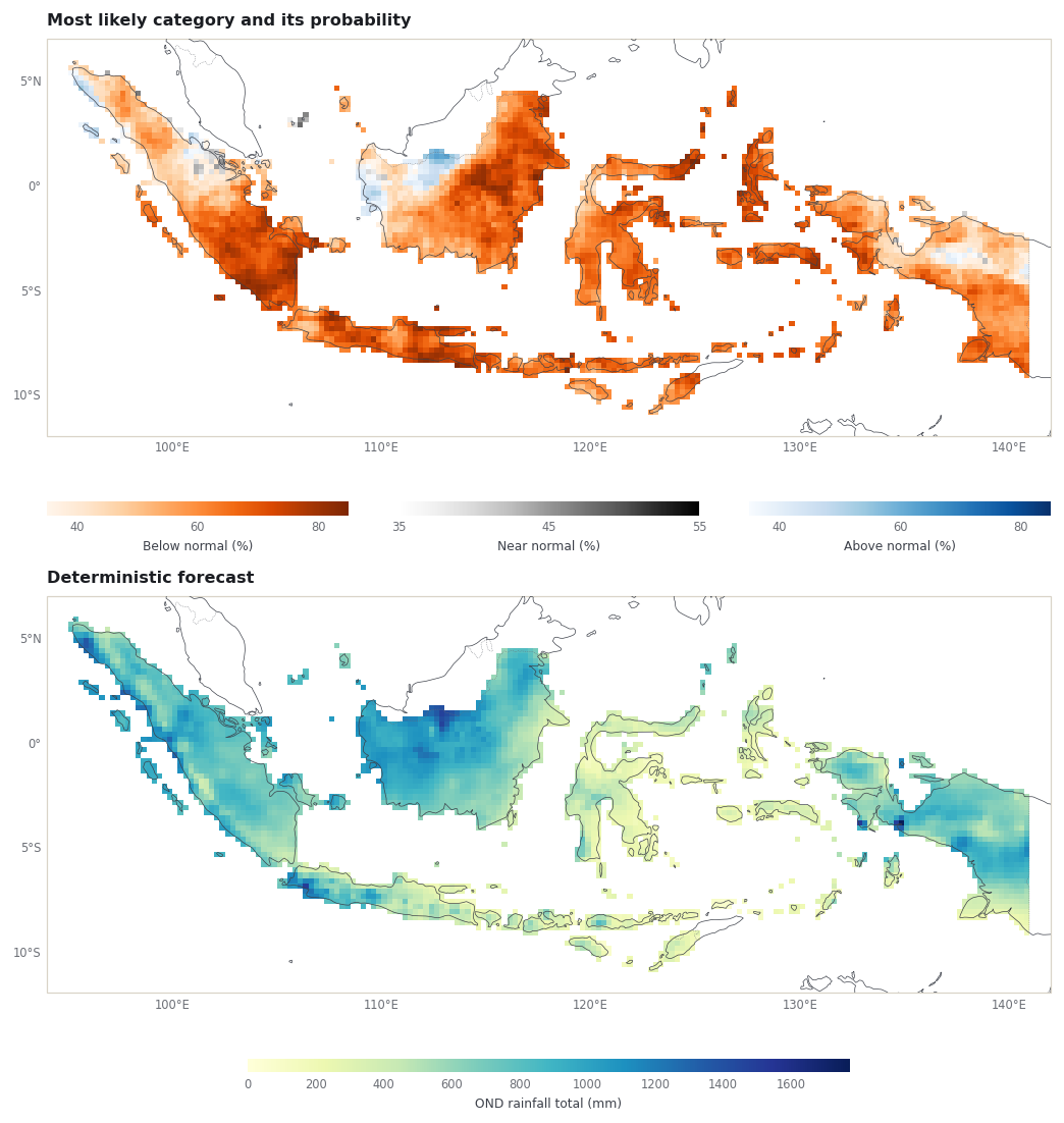
The same two maps as in chapter 4, now for the ensemble. The most-likely-category rule and colour ranges are PyCPT’s own (chapter 4, step 7).
mme_forecast = xr.Dataset({"deterministic": mme_det, "probabilistic": mme_prob})figures.forecast_figure(mme_forecast, predictand_box)plt.show()leading = [f.probabilistic.isel(T=0).fillna(-1).argmax("C").where(cells) for f in fcsts]mme_leading = mme_prob.isel(T=0).fillna(-1).argmax("C").where(cells)agreeing =sum((lead == mme_leading).astype(int) for lead in leading).where(cells)print("Members whose most likely category matches the ensemble's, share of cells (%):")print(pd.Series({n: round(float((agreeing == n).sum() / cells.sum() *100), 1) for n inrange(len(fcsts) +1)}).to_string())
Members whose most likely category matches the ensemble's, share of cells (%):
0     0.0
1     0.0
2     0.3
3     0.9
4     1.5
5     3.8
6    30.7
7    62.8
In most cells the members agree with the ensemble’s most likely category: the last two rows above count the cells where six or all seven members do. Where fewer agree, the ensemble’s leading category rests on a split between models.
7. One season: how did each forecast do in 2023?
The observed OND 2023 totals (CHIRPS v3.0, from the Fit & diagnose case) give one more comparison. As in chapter 5, one season is a description, not a skill test.
context = xr.open_dataset(repo /"docs/data/fitting-2023/comparison-context.nc")observed = context.observed_rainfall.sel(season="OND").reset_coords(drop=True)def rmse_2023(forecast): error = (forecast.isel(T=0) - observed).where(cells)returnfloat(np.sqrt((error **2).weighted(weights).mean(("Y", "X"))))season_table = pd.DataFrame( [{"forecast": n, "2023 RMSE (mm)": rmse_2023(f.deterministic)} for n, f inzip(predictor_names, fcsts)]+ [{"forecast": "MME (7 models)", "2023 RMSE (mm)": rmse_2023(mme_det)}]).set_index("forecast")season_table.round(1)
2023 RMSE (mm)
forecast
CFSv2.PRCP
124.1
CCSM4.PRCP
129.4
CESM1.PRCP
126.5
CanSIPSIC3.PRCP
124.1
GEOSS2S.PRCP
141.8
SEAS51c.PRCP
131.2
SPEAR.PRCP
176.1
MME (7 models)
131.6
In 2023 the ensemble’s error sits among its members’ errors rather than below all of them. A single season can favour any member; the 30-season cross-validated comparison above is the stronger evidence, and even that is limited to this domain, season and setup.
What you have now
A stated rule for choosing ensemble members, and the evidence for each candidate.
Seven models calibrated with identical settings by evaluate_models.
construct_mme read and checked: an equal-weight mean of the calibrated members, with in-sample probabilistic scores.
A measured comparison: lowest cross-validated error for the ensemble, but not the best on every measure or in every season.
The next chapter collects what changes when you adapt this workflow to your own region and season.
IRI Data Library. North American Multi-Model Ensemble (NMME) collection. https://iridl.ldeo.columbia.edu/SOURCES/.Models/.NMME/ Browsing Data Library pages requires signing in (checked 10 November 2026); PyCPT’s data requests in this tutorial succeeded without a key.
Kirtman, B., Min, D., Infanti, J., et al. (2014). The North American Multimodel Ensemble: Phase-1 seasonal-to-interannual prediction; Phase-2 toward developing intraseasonal prediction. Bulletin of the American Meteorological Society, 95(4), 585-601. https://doi.org/10.1175/BAMS-D-12-00050.1
Saha, S., Moorthi, S., Wu, X., et al. (2014). The NCEP Climate Forecast System Version 2. Journal of Climate, 27(6), 2185-2208. https://doi.org/10.1175/JCLI-D-12-00823.1
Johnson, S., Stockdale, T., Ferranti, L., et al. (2019). SEAS5: the new ECMWF seasonal forecast system. Geoscientific Model Development, 12, 1087-1117. https://doi.org/10.5194/gmd-12-1087-2019
Climate Hazards Center, UC Santa Barbara. CHIRPS: Rainfall Estimates from Rain Gauge and Satellite Observations (CHIRPS version 3.0 page). https://www.chc.ucsb.edu/data/chirps3
Funk, C., Peterson, P., Landsfeld, M., et al. (2014). A quasi-global precipitation time series for drought monitoring. U.S. Geological Survey Data Series 832. https://doi.org/10.3133/ds832