Prepare CHIRPS v3.0 seasonal totals and give them to PyCPT
The catalog offers a fixed list of observation datasets. PyCPT’s download_data also accepts a local predictand file in place of a catalog name; IRI’s operational template exposes this as local_predictand_file.
This chapter prepares OND rainfall totals from a local CHIRPS v3.0 archive, the observation product used by the case studies, and passes them to PyCPT. It then checks the result twice: against the observation file of the Fit & diagnose case, and against the CHIRPS v2.0 data downloaded in chapter 2.
NoteWhat you need to run this page
The full PyCPT environment, the case folder from chapters 1 and 2, and a local CHIRPS v3.0 file of 3-month rainfall totals (step 2 describes the one used here; point chirps3_file at your own copy). The country boundary comes from Natural Earth through Cartopy, which downloads it the first time it is used.
1. Repeat the case settings
The settings are unchanged. This time force_download=False: chapter 2 already downloaded the model data for exactly this question into this case folder, so reusing those files is correct. Chapter 1 explains why that is only safe when the folder and the question match.
from pathlib import Pathimport datetime as dtimport jsonimport osimport sysimport timeimport matplotlib.pyplot as pltimport numpy as npimport pandas as pdimport shapelyimport xarray as xrimport cartopy.io.shapereader as shapereaderimport pycptrepo =next((p for p in (Path.cwd(), *Path.cwd().parents) if (p /"pycpt_tutorial").is_dir()), None)if repo isNone:raiseFileNotFoundError("Run this notebook inside the tutorial repository or kit.")sys.path.insert(0, str(repo))from pycpt_tutorial.country_grid import aggregate_country_rainfall, training_complete_maskfrom pycpt_tutorial.export import save_netcdffrom pycpt_tutorial import figuresfigures.use_style()MOS ="CCA"predictor_names = ["CFSv2.PRCP"]download_args = {"fdate": dt.datetime(2023, 9, 1),"target": "Oct-Dec","target_first_year": 1991,"target_final_year": 2020,"predictor_extent": {"west": 85, "east": 155, "south": -20, "north": 20},"predictand_extent": {"west": 94, "east": 142, "south": -12, "north": 7},}force_download =Falsecase_dir = Path.home() /"PyCPT"/"indonesia-ond-2023-sep-init"domain_dir = pycpt.setup(case_dir, download_args["predictor_extent"])training_years =list(range(download_args["target_first_year"], download_args["target_final_year"] +1))
Input data will be saved in ~/PyCPT/indonesia-ond-2023-sep-init/85W-155E_to_-20S-20N/data
Figures will be saved in ~/PyCPT/indonesia-ond-2023-sep-init/85W-155E_to_-20S-20N/figures
Output will be saved in ~/PyCPT/indonesia-ond-2023-sep-init/85W-155E_to_-20S-20N/output
2. Open the local CHIRPS v3.0 file
The file used here holds 3-month rainfall totals at the native CHIRPS v3.0 resolution of 0.05°, one window every dekad from 1981 to 2025. It was built from the CHIRPS v3.0 global dekadal data distributed by the Climate Hazards Center. The cell prints the file’s own description rather than restating it.
chirps3_file = Path(os.environ.get("CHIRPS3_MONTH3_FILE","/mnt/e/temp/chirps/rolling_dekad/wld_cli_chirps3_month3_bydekad_1981_2025.nc"))source = xr.open_dataset(chirps3_file)print(f"File size: {chirps3_file.stat().st_size /1e9:.1f} GB")for key in ["title", "summary", "source", "version", "comment", "history"]:print(f"{key:>8}: {source.attrs.get(key)}")print()print("precip units:", source.precip.attrs.get("units"),"| grid:", f"{source.sizes['lat']} x {source.sizes['lon']}","| time steps:", source.sizes["time"])
File size: 24.3 GB
   title: CHIRPS Version 3.0 - 3-month precipitation accumulation, rolling by dekad
 summary: 3-month (9 dekad) rolling precipitation accumulation derived from CHIRPS v3.0 dekadal data, advancing one dekad at a time.
  source: CHIRPS v3.0 global dekad, Climate Hazards Center, UC Santa Barbara
 version: Version 3.0
 comment: Time stamp denotes the first day of the last dekad in the accumulation window; time_bnds spans the whole window.
 history: 2026-08-24T21:53:55 compute_rolling_multi(): 9-dekad rolling sum of wld_cli_chirps3_dekad_1981_2025.nc (nan_policy=strict)

precip units: mm | grid: 2400 x 7200 | time steps: 1612
3. Pick the OND windows by their bounds
The file’s comment says each time stamp is the first day of the last dekad in the window, and time_bnds gives the whole window. An OND total is therefore stamped 21 December. Rather than trusting that reasoning, the cell selects those stamps and checks that every window runs from 1 October to 1 January (end exclusive).
times = pd.DatetimeIndex(source.time.values)stamps = [int(np.flatnonzero((times.year == y) & (times.month ==12) & (times.day ==21))[0])for y in training_years]bounds = pd.DataFrame(source.time_bnds.isel(time=stamps).values, columns=["start", "end (exclusive)"])bounds.index = training_yearsexpected_start = pd.to_datetime([f"{y}-10-01"for y in training_years])expected_end = pd.to_datetime([f"{y +1}-01-01"for y in training_years])assert (bounds["start"].values == expected_start.values).all()assert (bounds["end (exclusive)"].values == expected_end.values).all()print(f"All {len(stamps)} windows span 1 October to 31 December of their year.")bounds.iloc[[0, 1, -1]]
All 30 windows span 1 October to 31 December of their year.
start
end (exclusive)
1991
1991-10-01
1992-01-01
1992
1992-10-01
1993-01-01
2020
2020-10-01
2021-01-01
4. Read only the predictand box
The file is large, but only 30 time steps inside the predictand box are needed. xarray reads just that subset from disk.
Read {'time': 30, 'lat': 380, 'lon': 960} in 8 s
Longitude 94.025 to 141.975, latitude -11.975 to 6.975
Negative values: 0 | missing values: 7886640
5. Aggregate 0.05° to the 0.25° grid over Indonesia
The predictand grid matches the case studies: 0.25° cells whose centres run from 94.125°E and 6.875°N. Each 0.25° cell holds 5 × 5 native pixels. The case studies used the tutorial’s helper aggregate_country_rainfall, which:
keeps only native pixels whose centres fall inside Indonesia,
averages them with cos(latitude) area weights, so a cell value is a mean rainfall depth, not a sum over pixels,
keeps a cell only if at least 99% of its Indonesian land weight has data.
The boundary is the Natural Earth 1:10m country polygon for Indonesia (ADM0_A3 = IDN).
records = shapereader.Reader(shapereader.natural_earth("10m", "cultural", "admin_0_countries")).records()indonesia =next(r.geometry for r in records if r.attributes["ADM0_A3"] =="IDN")shapely.prepare(indonesia)lon2d, lat2d = np.meshgrid(native.lon, native.lat)country = xr.DataArray(shapely.contains_xy(indonesia, lon2d, lat2d), dims=("lat", "lon"), coords={"lat": native.lat, "lon": native.lon})print(f"Native pixels inside Indonesia: {int(country.sum()):,} of {country.size:,}")centres_y = box["south"] +0.125+ np.arange(76) *0.25centres_x = box["west"] +0.125+ np.arange(192) *0.25seasons = []for i inrange(native.sizes["time"]): block = aggregate_country_rainfall(native.isel(time=i, drop=True), country, 5, minimum_coverage=0.99) seasons.append(block.precipitation.rename({"lat": "Y", "lon": "X"}) .assign_coords(Y=centres_y, X=centres_x).sortby("Y", ascending=False))
Native pixels inside Indonesia: 61,192 of 364,800
The case studies kept only cells with data in every training season. The same rule is applied here, so the two results can be compared directly.
The target dates T, Ti and Tf are copied from the CFSv2 hindcasts downloaded in chapter 2, which makes the alignment of model and observation seasons explicit. The hindcasts’ initialization date S is not copied: observations have no initialization, and PyCPT’s own downloaded observations carry no S. This matters in practice. A first version of this file inherited S from the model time axis; it passed cptio’s checks, but in this environment the fit in chapter 4 then failed while reading CPT’s output, because CPT 17.8.3 wrote the initialization date without a time and cptio 1.4.0 refuses such dates.
hindcasts = xr.open_dataset(domain_dir /"data"/"CFSv2.PRCP.nc")model_time = pd.Index(hindcasts["T"].values, name="T")assert (model_time.year == np.array(training_years)).all()chirps3 = (xr.concat(seasons, dim=model_time) .assign_coords(Ti=("T", hindcasts["Ti"].values), Tf=("T", hindcasts["Tf"].values)))assert"S"notin chirps3.coordscomplete = training_complete_mask(chirps3, training_years)chirps3 = chirps3.where(complete).transpose("T", "Y", "X").rename("precipitation")chirps3.attrs = {"units": "mm", "missing": -999.0,"long_name": "CHIRPS v3.0 OND rainfall total, Indonesia land, 0.25 degree"}print(f"Cells with data in all {len(training_years)} seasons: {int(complete.sum())}")print("Season of first value:", str(chirps3["Ti"].values[0])[:10], "to", str(chirps3["Tf"].values[0])[:10])print(f"Range: {float(chirps3.min()):.1f} to {float(chirps3.max()):.1f} mm")
Cells with data in all 30 seasons: 3240
Season of first value: 1991-10-01 to 1991-12-31
Range: 5.8 to 3470.0 mm
6. Save the file and give it to PyCPT
download_data accepts a local file ending in .nc (opened with xarray) or .tsv (CPT text). It takes the first data variable in the file, so the file should contain only the rainfall variable. The file name is chosen so it cannot collide with PyCPT’s own download names.
download_data itself does not check the file. The check happens later, when cptcore starts a fit and calls cptio’s is_valid_cptv10_xyt on the predictand. In the installed cptio 1.4.0 that check requires, among other things:
T, Y and X coordinates, and only coordinates from CPT’s list (T, Ti, Tf, S, X, Y and a few others);
Ti and Tf together or not at all;
a units attribute;
a missing attribute holding a number, the value CPT writes in place of NaN.
The first version of this chapter left out missing, and the fit in chapter 4 stopped with that assertion. The attribute is set above, and the cell after the load runs the same check that cptcore will run.
local_predictand_file = domain_dir /"data"/"local-CHIRPS3-OND-1991-2020.nc"save_netcdf(chirps3.to_dataset(), local_predictand_file, overwrite=True, metadata={"source_file": chirps3_file.name,"aggregation": "cos-latitude weighted mean of Indonesian 0.05 degree pixels per 0.25 degree cell; at least 99% country-land coverage","boundary": "Natural Earth 1:10m admin_0_countries, ADM0_A3=IDN","training_years": "1991-2020"})Y, hindcast_data, forecast_data = pycpt.download_data("CHIRPS3 (local)", local_predictand_file, predictor_names, download_args, domain_dir, force_download)print("Data variable PyCPT took:", Y.name, "| shape:", dict(Y.sizes))
Reusing already-downloaded CFSv2.PRCP_f2023

Using local observed predictand dataset
Reusing already-downloaded CFSv2.PRCP

Data variable PyCPT took: precipitation | shape: {'T': 30, 'Y': 76, 'X': 192}
from cptio.utilities.verify import is_valid_cptv10_xytis_valid_cptv10_xyt(Y)print("Passes cptio's CPTv10 check, the one cptcore runs before fitting.")print("units:", Y.attrs["units"], "| missing:", Y.attrs["missing"], "| coordinates:", sorted(Y.coords))
Passes cptio's CPTv10 check, the one cptcore runs before fitting.
units: mm | missing: -999.0 | coordinates: ['T', 'Tf', 'Ti', 'X', 'Y']
pycpt.summarize_available_years(predictor_names, "CHIRPS3 (local)", download_args,
                                Y, hindcast_data, forecast_data)
Training data
Observations were retrieved for all years of the training period.
Hindcasts were retrieved for all years of the training period.
CHIRPS3 (local)
CFSv2.PRCP
1991
ok
ok
1992
ok
ok
1993
ok
ok
1994
ok
ok
1995
ok
ok
1996
ok
ok
1997
ok
ok
1998
ok
ok
1999
ok
ok
2000
ok
ok
2001
ok
ok
2002
ok
ok
2003
ok
ok
2004
ok
ok
2005
ok
ok
2006
ok
ok
2007
ok
ok
2008
ok
ok
2009
ok
ok
2010
ok
ok
2011
ok
ok
2012
ok
ok
2013
ok
ok
2014
ok
ok
2015
ok
ok
2016
ok
ok
2017
ok
ok
2018
ok
ok
2019
ok
ok
2020
ok
ok
Forecast data
All forecasts were retrieved.
CFSv2.PRCP
2023
ok
7. Check against the Fit & diagnose observations
The case study prepared its observations with a separate research script from the same CHIRPS v3.0 archive. If both routes are right, the arrays must be identical.
Same missing-value pattern: True
Same target dates: True
Largest difference: 0.0 mm
The predictand built here is the Fit & diagnose predictand, value for value. Any difference in the next chapter’s fits will therefore come from the predictor: chapter 2 measured how PyCPT’s CFSv2 totals differ from the case study’s.
8. CHIRPS v3.0 or v2.0: does the choice matter?
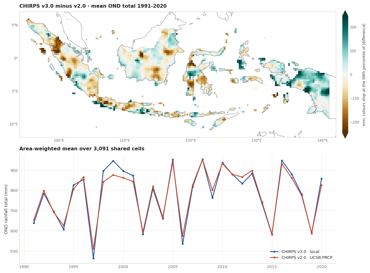
Chapter 2 downloaded the catalog’s CHIRPS v2.0 (UCSB.PRCP) on the same 0.25° grid. The two fields are compared only on cells where both have data in every training season. Two things differ at once: the product version, and the way each 0.25° value was made (the Data Library’s 0.25° CHIRPS v2.0 grid versus the Indonesia-only average built here). The comparison shows the combined effect; it does not separate them.
ucsb = xr.open_dataset(domain_dir /"data"/"UCSB.PRCP.nc").prcpassert np.allclose(ucsb["X"], Y["X"]) and np.allclose(ucsb["Y"], Y["Y"])assert (ucsb["T"].values == Y["T"].values).all()v3_all = Y.transpose("T", "Y", "X")v2_all = ucsb.transpose("T", "Y", "X")v3_complete = v3_all.notnull().all("T")both = v3_complete & v2_all.notnull().all("T")shared_cells =int(both.sum())print(f"CHIRPS v3.0 cells kept above: {int(v3_complete.sum())}")print(f"Of those, cells where CHIRPS v2.0 also has data in every season: {shared_cells}")print(f"Cells with v3.0 data but no complete v2.0 series: {int((v3_complete &~both).sum())}")v3 = v3_all.where(both)v2 = v2_all.where(both)weights = np.cos(np.deg2rad(v3["Y"])) * bothnational_v3 = v3.weighted(weights).mean(("Y", "X"))national_v2 = v2.weighted(weights).mean(("Y", "X"))difference = v3 - v2summary = pd.Series({"national mean OND total, v3.0 (mm)": float(national_v3.mean()),"national mean OND total, v2.0 (mm)": float(national_v2.mean()),"mean difference v3.0 - v2.0 (mm)": float((national_v3 - national_v2).mean()),"correlation of yearly national totals": float(np.corrcoef(national_v3, national_v2)[0, 1]),"median absolute cell difference (mm)": float(np.nanmedian(np.abs(difference))),"95th percentile absolute cell difference (mm)": float(np.nanpercentile(np.abs(difference), 95)),}).round(3)summary.to_frame("value")
CHIRPS v3.0 cells kept above: 3240
Of those, cells where CHIRPS v2.0 also has data in every season: 3091
Cells with v3.0 data but no complete v2.0 series: 149
value
national mean OND total, v3.0 (mm)
781.289
national mean OND total, v2.0 (mm)
780.697
mean difference v3.0 - v2.0 (mm)
0.592
correlation of yearly national totals
0.986
median absolute cell difference (mm)
73.275
95th percentile absolute cell difference (mm)
267.897
fig, grid = figures.stacked([figures.map_height(figures.extent_of(box)), 3.2])mean_diff = difference.mean("T")limit =float(np.nanpercentile(np.abs(mean_diff), 98))ax = figures.map_axes(fig, grid[0, 0], figures.extent_of(box))image = figures.draw_field(ax, mean_diff, cmap="BrBG", vmin=-limit, vmax=limit)ax.set_title("CHIRPS v3.0 minus v2.0 · mean OND total 1991-2020")figures.colorbar(fig, image, ax, "mm; colours stop at the 98th percentile of |difference|", extend="both")ax = fig.add_subplot(grid[1, 0])years = v3["T"].dt.yearax.plot(years, national_v3, marker="o", markersize=3, label="CHIRPS v3.0 · local")ax.plot(years, national_v2, marker="o", markersize=3, label="CHIRPS v2.0 · UCSB.PRCP")ax.set_title(f"Area-weighted mean over {shared_cells:,} shared cells")ax.set_ylabel("OND rainfall total (mm)")ax.legend(loc="lower right")plt.show()
Read the numbers above before choosing. A choice of observations changes what the calibration learns and what it is scored against, so it should be made for a documented reason, such as the product a national service already uses, and not by comparing which one gives better skill.
What you have now
A local CHIRPS v3.0 OND predictand built from a documented archive, with each window checked by its time bounds.
The file loaded through PyCPT’s local_predictand_file option, with every training year present.
Proof that it equals the Fit & diagnose predictand.
A measured comparison with the catalog’s CHIRPS v2.0.
The next chapter fits CCA with evaluate_models on these inputs and compares the result with the Fit & diagnose case.
Climate Hazards Center, UC Santa Barbara. CHIRPS: Rainfall Estimates from Rain Gauge and Satellite Observations (CHIRPS version 3.0 page). https://www.chc.ucsb.edu/data/chirps3
Funk, C., Peterson, P., Landsfeld, M., et al. (2014). A quasi-global precipitation time series for drought monitoring. U.S. Geological Survey Data Series 832. https://doi.org/10.3133/ds832
IRI Data Library. UCSB CHIRPS version 2.0. https://iridl.ldeo.columbia.edu/SOURCES/.UCSB/.CHIRPS/.v2p0/ Browsing Data Library pages requires signing in (checked 10 November 2026); PyCPT’s data requests in this tutorial succeeded without a key.
Funk, C., Peterson, P., Landsfeld, M., et al. (2015). The climate hazards infrared precipitation with stations: a new environmental record for monitoring extremes. Scientific Data, 2, 150066. https://doi.org/10.1038/sdata.2015.66